Estimating averages from sparse samples¶

A satellite instrument samples the atmosphere along its orbit: unevenly in latitude, longitude and time, with gaps. Averaging whatever falls in a latitude bin into a “monthly zonal mean” silently weights the days, longitudes and latitudes that happened to be sampled, which biases the result wherever the field varies over the month. optimal_estimate() instead computes the best linear unbiased estimate of each average (kriging), its uncertainty, and the weights that show how it was obtained.

The estimate¶

Observations \(y_k\) are averages of the field \(f\) over product kernels (points, or footprints and time windows given as spaces) with noise variances \(\epsilon_k\). Targets \(g_m\) are averages over a grid of product elements, optionally area weighted. With a prior covariance \(C(x, x') = \sigma^2 \prod_d c_d(x_d - x'_d)\) and a mean \(\mu(x) = \sum_p \beta_p h_p(x)\) with unknown coefficients,

\[ \hat g = H_t \hat\beta + B Q^{-1} (y - H \hat\beta), \qquad \hat\beta = (H^\top Q^{-1} H)^{-1} H^\top Q^{-1} y, \qquad Q = C_{oo} + \operatorname{diag}(\epsilon), \]

where \(B\) is the target–observation covariance and \(H\), \(H_t\) the mean basis averaged like the observations and targets. Every covariance is computed exactly: a month against a point, a latitude band against a latitude band, with the cos-latitude area weight, around a periodic longitude. The posterior variance includes the uncertainty of \(\hat\beta\).

Choosing the pieces:

Covariance (Covariance): per dimension a CovarianceDim with family "squared_exponential", "exponential", "matern32" or "matern52", a correlation length, optionally a period (longitude), and optionally a VarianceProfile s(x) (a spline) for variability that changes along the dimension, e.g. peaking at a polar vortex edge: the covariance becomes s(x) s(x’) ρ(x − x’), still integrated exactly. Sums of covariances (CovarianceSum) combine scales. Fit the variance and lengths by maximizing log_likelihood (see log_likelihood()).
Mean: "estimate" for an unknown constant, a dict of spaces for a structured mean that is reproduced exactly, or a list of MeanTerm whose coefficients are either unconstrained or given a Gaussian prior. Where data are missing the estimate relaxes towards the mean, so a mean with the field’s large-scale structure matters there; a prior on terms the data only partly determine (a drift through a month sampled in its first half, structure beyond the data’s latitudes) keeps them from being extrapolated. Periodic bases, harmonics() (zonal waves, annual cycles) and bsplines_periodic(), give the mean structure in longitude: with waves in the mean, a field that is a sum of waves has its zonal mean recovered exactly even from a single longitude sector.
Several quantities at once: values of shape (n, k), e.g. one column per altitude, share the covariance and, for columns with the same valid observations, its factorization. Normalize the columns (e.g. by their means) when one covariance should describe them all.

Example: a month of limb-sounder data¶

A synthetic field with a latitude structure that drifts through the month and a travelling planetary wave, sampled by a sun-synchronous instrument: 14 orbits a day, an outage for the last ten days, and northern high latitudes that leave the sunlit field of view after day 8.

import matplotlib.pyplot as plt
import numpy as np

import rebasis as rb
from _plot import BLUE, MUTED, ORANGE

rng = np.random.default_rng(1)


def field(lat, lon, t):
    r = np.radians(lat)
    zonal = 250 + 40 * np.cos(r) ** 2 + 0.8 * t * np.sin(r)  # drifts through the month
    wave = 10 * np.cos(r) ** 2 * np.sin(np.radians(2 * lon) - 0.25 * t)
    return zonal + wave


lat, lon, t = [], [], []
for day in range(20):  # outage from day 20
    for orbit in range(14):
        lon0 = (180 - 25.7 * (day * 14 + orbit)) % 360
        for la in np.arange(-80, 81, 3.0):
            if la > 50 and day >= 8:  # out of the sunlit field of view
                continue
            lat.append(la + rng.normal(0, 0.5))
            lon.append((lon0 + 0.2 * la) % 360)
            t.append(day + orbit / 14 + (la + 90) / 180 * 0.5 / 14)
lat, lon, t = map(np.array, (lat, lon, t))
y = field(lat, lon, t) + rng.normal(0, 2.0, lat.size)
print(f"{y.size} observations")

13440 observations

The true area-weighted zonal monthly means, in closed form (the wave averages out over longitude):

edges = np.arange(-80, 81, 10.0)
s = np.sin(np.radians(edges))
ds = np.diff(s)
truth = (250 * ds + 40 * np.diff(s - s**3 / 3) + 0.8 * 15 * np.diff(s**2 / 2)) / ds
centers = 0.5 * (edges[1:] + edges[:-1])

The estimate: monthly means over 10° bands, all longitudes, days 0-30, with a mean that is a smooth function of latitude drifting linearly in time.

cov = rb.Covariance(
    30.0,
    lat=rb.CovarianceDim("squared_exponential", 10.0),
    lon=rb.CovarianceDim("exponential", 90.0, period=360.0),
    time=rb.CovarianceDim("matern32", 6.0),
)
est = rb.optimal_estimate(
    y,
    {"lat": lat, "lon": lon, "time": t},
    {"lat": rb.Space.boxes(edges), "lon": rb.Space.boxes([0, 360]), "time": rb.Space.boxes([0, 30])},
    cov,
    noise=2.0**2,
    target_weight={"lat": "cos_lat_deg"},
    mean={"lat": rb.Space.bsplines_clamped(np.linspace(-90, 90, 7), 3), "time": rb.Space.hats([0.0, 30.0])},
)
bin_average = np.array([y[(lat >= a) & (lat < b)].mean() for a, b in zip(edges[:-1], edges[1:])])

fig, ax = plt.subplots(figsize=(8, 3.4))
ax.axhline(0, color=MUTED, lw=1)
ax.plot(centers, bin_average - truth, "o", color=ORANGE, label="bin average − truth")
ax.errorbar(centers, est.values[:, 0, 0] - truth, yerr=2 * est.std[:, 0, 0], fmt="o", color=BLUE,
            capsize=3, label="optimal estimate − truth (± 2σ)")
ax.set_xlabel("latitude band center [°]")
ax.set_ylabel("error")
ax.legend(loc="lower left");

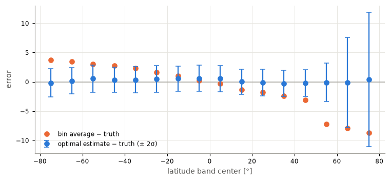
_images/bfd4ccede8622961e174ebeeaf60b395a74fd90418e4991b3e3b7c1f390d1c82.png

Bin averages are biased by the outage wherever the field drifts (the poles) and by the lost northern coverage; the optimal estimate removes most of that bias, and its uncertainty grows where data are missing.

Where the weights go¶

weight_histogram() sums each target’s weights over the observations by day. A monthly mean should weight every day equally (1/30); the bin average can only weight the days that were sampled.

days = np.arange(0, 31)
w = est.weight_histogram(t, days)
fig, axes = plt.subplots(1, 2, figsize=(9, 3), sharey=True)
for ax, band in zip(axes, [8, 14]):
    sel = (lat >= edges[band]) & (lat < edges[band + 1])
    naive = np.histogram(t[sel], days)[0] / sel.sum()
    ax.stairs(naive, days, color=ORANGE, label="bin average")
    ax.stairs(w[band, 0, 0], days, color=BLUE, label="optimal estimate")
    ax.axhline(1 / 30, color=MUTED, lw=1, ls="--", label="ideal (1/30 per day)")
    ax.set_title(f"{edges[band]:.0f}° to {edges[band + 1]:.0f}°", loc="left")
    ax.set_xlabel("day")
axes[0].set_ylabel("weight per day")
axes[0].legend(loc="upper right")
print("each band's weights sum to", np.round(est.weights.sum(axis=1), 12)[:3], "...")

each band's weights sum to [1. 1. 1.] ...

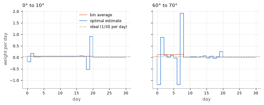
_images/9339d1a67f03121bdaf50531c63373bdfd8e33d15dcd417c015e06f2bfe4e674.png

The large positive and negative weights at the ends of each sampled period are how the estimate extrapolates the mean’s linear drift into the gap: a difference between early and late data, scaled to reach the middle of the month. That is what removes the bias, and it is exactly as good as the assumption that the drift is linear; the posterior uncertainty accounts for the estimated drift but not for a wrong mean model. The weights in each band still sum to one, and any field in the span of the mean basis is reproduced exactly.

Fitting the covariance¶

fit_covariance() maximizes the (restricted) log likelihood over the variance and correlation lengths, a nugget added to the noise, and the widths of mean terms with priors, with analytic gradients (the length derivatives of every covariance, box averages included, are exact). A subsample of a few thousand observations usually determines them well:

drift = rb.Space.shifted([15.0], [-15.0, 15.0], [-0.5, 0.5])  # (t − 15) / 30
lat_basis = rb.Space.bsplines_clamped(np.linspace(-90, 90, 7), 3)
fit = rb.fit_covariance(
    y,
    {"lat": lat, "lon": lon, "time": t},
    cov,
    noise=2.0**2,
    mean=[rb.MeanTerm({"lat": lat_basis}), rb.MeanTerm({"lat": lat_basis, "time": drift}, prior_std=1.0)],
    subsample=1500,
)
print(fit.success, fit.n_iterations, "iterations")
{k: round(v, 3) for k, v in fit.parameters.items()}

True 38 iterations

{'variance': 22.565,
 'length.lat': 49.304,
 'length.lon': 72.188,
 'length.time': 6.369,
 'mean.1.prior_std': 0.03,
 'nugget': 0.0}

fit.estimate(...) then runs optimal_estimate() with the fitted covariance, mean and nugget.

Cost and neighbourhoods¶

The n × n observation covariance is formed in Rust and factored with LAPACK (O(n³)); the posterior variances need one solve per target. This example (\(n \approx 13\,000\)) takes a few seconds.

For more data, estimate locally: neighborhood={"lat": 10, "time": 5} groups the targets into blocks (here each latitude band × month) and estimates each block from the observations within 10° of latitude and 5 days of its targets. The cost then grows with the neighbourhood, not the data set: a year of 50 000 observations, as monthly 10° zonal means, takes a few seconds. Choose half widths of a few correlation lengths, beyond which observations carry little weight; n_used reports how many observations each estimate drew on.