Quickstart

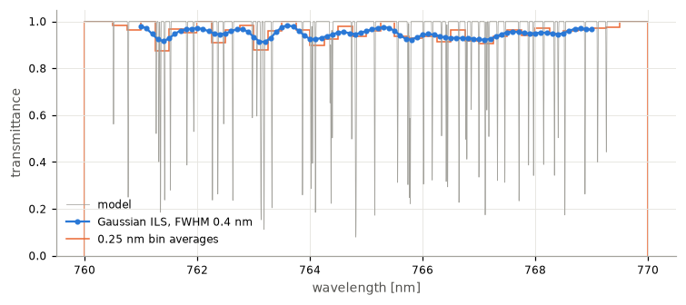
A synthetic high-resolution transmittance spectrum, measured by an instrument with a Gaussian line shape, then regridded conservatively onto coarse bins.

import matplotlib.pyplot as plt
import numpy as np

import rebasis as rb
from _plot import BLUE, MUTED, ORANGE

rng = np.random.default_rng(3)
x = np.linspace(760.0, 770.0, 20001)  # model grid [nm], 0.0005 nm sampling
lines = rng.uniform(760.5, 769.5, 60)
tau = sum(d * np.exp(-0.5 * ((x - c) / 0.004) ** 2) for c, d in zip(lines, rng.uniform(0.2, 0.9, 60)))
f = np.exp(-2 * tau)

The model values are samples, so the spectrum is represented in the hat (piecewise-linear) basis: its coefficients are the samples and the function is their linear interpolant.

hires = rb.Space.hats(x)
hires

Space(hats, n=20001, support=[760, 770])

Measuring with an instrument line shape

Kernels are a space too. measure() returns a sparse matrix whose row \(i\) holds \(\int K_i B_j / \int K_i\): each channel is a unit-area weighted average of the spectrum.

centers = np.arange(761.0, 769.01, 0.1)
ils = rb.Space.gaussians(centers, fwhm=0.4)
W = rb.measure(ils, hires)
print(type(W).__name__, W.shape, f"{W.nnz:,} nonzeros")
measured = W @ f

csr_array (81, 20001) 330,321 nonzeros

Regridding

regrid() projects onto another basis. Onto boxes, the result is the bin average and the integral of the spectrum is conserved exactly.

edges = np.arange(760.0, 770.01, 0.25)
bins = rb.Space.boxes(edges)
binned = rb.regrid(f, hires, bins)
print("∫f model:", f @ hires.integrals(), " ∫f bins:", binned @ bins.integrals())

∫f model: 9.553967978067401  ∫f bins: 9.553967978067401

fig, ax = plt.subplots(figsize=(8, 3.2))
ax.plot(x, f, color=MUTED, lw=0.5, label="model")
ax.plot(centers, measured, ".-", color=BLUE, label="Gaussian ILS, FWHM 0.4 nm")
ax.stairs(binned, edges, color=ORANGE, label="0.25 nm bin averages")
ax.set_xlabel("wavelength [nm]")
ax.set_ylabel("transmittance")
ax.legend(loc="lower left");