Line shapes

Every constructor takes the line centers and per-element (or shared) width parameters. All shapes peak at 1; measure() normalizes them to unit area. cutoff is the half width of the truncated support in the unit given.

constructor	shape	cutoff unit (default)
gaussians()	Gaussian	σ (6)
lorentzians()	Lorentzian	HWHM (100)
voigts()	Voigt, via the Faddeeva function	Voigt HWHM (100)
pseudo_voigts()	η·Lorentzian + (1 − η)·Gaussian	HWHM (100)
super_gaussians()	exp(−ln 2·|2t/w|ᵖ), optionally asymmetric	HWHM per side (6)
smoothed_boxes()	slit ⊗ Gaussian	σ beyond the box edges (6)
fts()	FTS line shape for an apodization	1/(2·max OPD) (100)
rectangles(), triangles(), trapezoids()	piecewise linear
shifted()	one tabulated shape (linear or PCHIP), stored once
tabulated()	a tabulated shape per channel

FTS apodizations: "none" (sinc), "triangle" (sinc²), "hann", "hamming" (Happ–Genzel), "blackman", "blackman_harris", "norton_beer_weak", "norton_beer_medium", "norton_beer_strong", or custom cosine-sum or Norton–Beer coefficients.

Channels with different shapes (a Gaussian here, a tabulated shape there) form one space with concatenate(), so a whole instrument is still a single measure().

Show code cell source

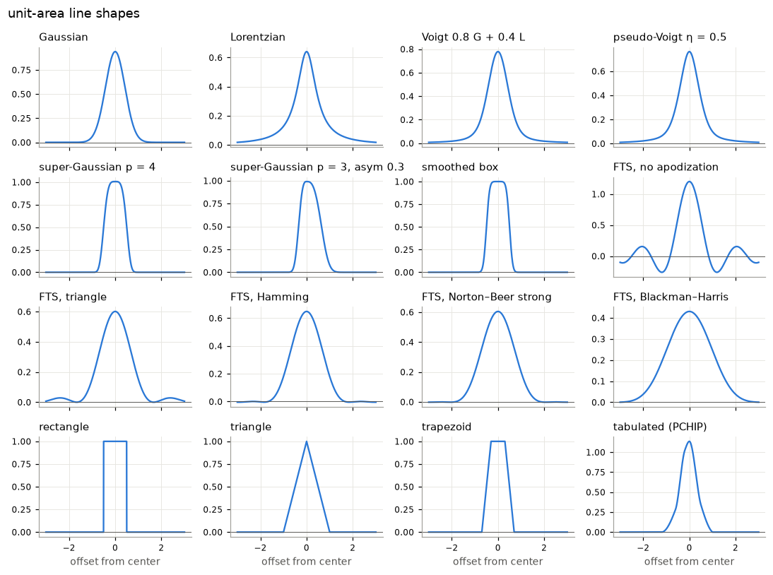
Hide code cell source

import matplotlib.pyplot as plt
import numpy as np

import rebasis as rb
from _plot import BLUE

c = [0.0]
shapes = [
    ("Gaussian", rb.Space.gaussians(c, fwhm=1.0)),
    ("Lorentzian", rb.Space.lorentzians(c, fwhm=1.0)),
    ("Voigt 0.8 G + 0.4 L", rb.Space.voigts(c, fwhm_gaussian=0.8, fwhm_lorentzian=0.4)),
    ("pseudo-Voigt η = 0.5", rb.Space.pseudo_voigts(c, fwhm=1.0, eta=0.5)),
    ("super-Gaussian p = 4", rb.Space.super_gaussians(c, fwhm=1.0, power=4)),
    ("super-Gaussian p = 3, asym 0.3", rb.Space.super_gaussians(c, fwhm=1.0, power=3, asymmetry=0.3)),
    ("smoothed box", rb.Space.smoothed_boxes(c, width=1.0, fwhm=0.25)),
    ("FTS, no apodization", rb.Space.fts(c, max_opd=0.6, apodization="none")),
    ("FTS, triangle", rb.Space.fts(c, max_opd=0.6, apodization="triangle")),
    ("FTS, Hamming", rb.Space.fts(c, max_opd=0.6, apodization="hamming")),
    ("FTS, Norton–Beer strong", rb.Space.fts(c, max_opd=0.6, apodization="norton_beer_strong")),
    ("FTS, Blackman–Harris", rb.Space.fts(c, max_opd=0.6, apodization="blackman_harris")),
    ("rectangle", rb.Space.rectangles(c, width=1.0)),
    ("triangle", rb.Space.triangles(c, fwhm=1.0)),
    ("trapezoid", rb.Space.trapezoids(c, top_width=0.6, bottom_width=1.4)),
    ("tabulated (PCHIP)", rb.Space.shifted(c, [-1.2, -0.6, -0.2, 0.0, 0.5, 1.0],
                                           [0, 0.25, 0.9, 1.0, 0.3, 0], interp="pchip")),
]
x = np.linspace(-3, 3, 1201)
fig, axes = plt.subplots(4, 4, figsize=(10, 7.5), sharex=True)
for ax, (title, s) in zip(axes.flat, shapes):
    ax.plot(x, s.evaluate(x).toarray()[:, 0] / s.integrals()[0], color=BLUE)
    ax.axhline(0, color="#52514e", lw=0.6)
    ax.set_title(title, loc="left")
for ax in axes[-1]:
    ax.set_xlabel("offset from center")
fig.suptitle("unit-area line shapes", x=0.01, ha="left")
fig.tight_layout()

Accuracy against independent references

The Voigt profile uses Weideman’s rational approximation of the Faddeeva function (order 40), accurate to about \(3\times10^{-15}\) of the peak value:

from scipy.special import voigt_profile

t = np.linspace(-3, 3, 601)
v = rb.Space.voigts([0.0], sigma=0.3, gamma=0.1, cutoff=1e4).evaluate(t).toarray()[:, 0]
ref = voigt_profile(t, 0.3, 0.1) / voigt_profile(0.0, 0.3, 0.1)
print(f"max |difference| from scipy: {np.abs(v - ref).max():.1e}")

max |difference| from scipy: 6.7e-16