Example: coated black carbon

Soot ages in the atmosphere by gathering a coating of sulfate, organics and water. The coating absorbs almost nothing itself, but it focuses light onto the absorbing core, so a coated particle absorbs more than its bare core: the absorption enhancement. This page computes it for single particles with scatrs.layered, then for a size distribution of coated particles with LayeredSphere, and differentiates the results with respect to the coating. See Layered spheres for the method. This page runs whenever the documentation is built; its checks are asserts, so a failing check fails the build.

The refractive indices are constants here: \(1.95 + 0.79i\) for black carbon (Bond & Bergstrom 2006) and \(1.43 + 10^{-8}i\) for sulfate. Radii and wavelengths are in µm.

import matplotlib.pyplot as plt
import numpy as np

import scatrs
from scatrs import layered

bc, sulfate = 1.95 + 0.79j, 1.43 + 1e-8j

One particle: the absorption enhancement

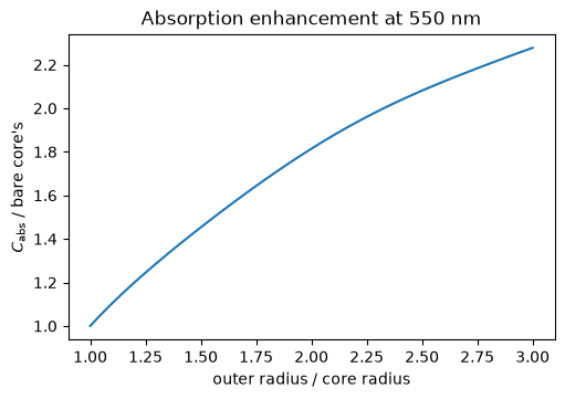
A black-carbon core of radius 0.05 µm, in sulfate shells of growing thickness, at 550 nm. The size parameters of the interfaces go along the last axis, the core’s first, and broadcast as in scatrs.mie. The absorption cross section is \(Q_\text{abs}\) times the geometric cross section of the outer surface.

wavelength, r_core = 0.55, 0.05
k = 2 * np.pi / wavelength
r_outer = r_core * np.linspace(1, 3, 41)  # the outer radius, from a bare core to 3 times it
x = np.stack([np.full_like(r_outer, k * r_core), k * r_outer], axis=-1)
q = layered.efficiencies(x, [bc, sulfate])
c_abs = q.q_abs * np.pi * r_outer**2
enhancement = c_abs / c_abs[0]
print(f"bare core: C_abs = {c_abs[0]:.3e} µm²")
for ratio in (1.5, 2.0, 3.0):
    i = np.argmin(abs(r_outer / r_core - ratio))
    print(f"outer/core radius {ratio}: enhancement {enhancement[i]:.2f}")
assert np.all(np.diff(enhancement) > 0) and 2 < enhancement[-1] < 2.5

bare core: C_abs = 6.005e-03 µm²
outer/core radius 1.5: enhancement 1.45
outer/core radius 2.0: enhancement 1.81
outer/core radius 3.0: enhancement 2.28

The first point is the bare core itself: a shell of zero thickness changes nothing. A coating twice the core’s radius nearly doubles the absorption, even though it absorbs almost nothing itself.

fig, ax = plt.subplots(figsize=(5, 3.5), layout="constrained")
ax.plot(r_outer / r_core, enhancement)
ax.set(xlabel="outer radius / core radius", ylabel="$C_\\mathrm{abs}$ / bare core's",
       title="Absorption enhancement at 550 nm")
plt.show()

A size distribution of coated particles

In an ensemble, the size distribution gives the outer radius, and each interface stays at a fixed fraction of it: here the core’s radius is 60% of the particle’s, so its volume fraction is \(0.6^3 \approx 0.22\). LayeredSphere.coated builds a core and one shell. The bare cores alone are an ensemble of spheres whose distribution is the coated one’s scaled by the fraction: a lognormal of median radius \(0.6\,r_g\) and the same width.

r_g, width, f = 0.08, 1.6, 0.6
wavelengths = np.array([0.35, 0.45, 0.55, 0.7, 0.87, 1.06])
coated = scatrs.Ensemble(
    scatrs.LayeredSphere.coated(bc, sulfate, core_fraction=f),
    scatrs.LogNormal(median_radius=r_g, width=width),
)
cores = scatrs.Ensemble(scatrs.Sphere(bc), scatrs.LogNormal(median_radius=f * r_g, width=width))
r, bare = coated.compute(wavelengths), cores.compute(wavelengths)
print(f"{'λ (µm)':>7}{'ω coated':>10}{'ω cores':>9}{'enhancement':>13}")
for row in zip(wavelengths, r.ssa, bare.ssa, r.c_abs / bare.c_abs, strict=True):
    print("{:7.2f}{:10.3f}{:9.3f}{:13.2f}".format(*row))
assert r.converged.all() and bare.converged.all()
assert np.all(r.c_abs / bare.c_abs > 1.4) and np.all(r.ssa > bare.ssa)

 λ (µm)  ω coated  ω cores  enhancement
   0.35     0.551    0.408         1.65
   0.45     0.522    0.372         1.61
   0.55     0.497    0.337         1.59
   0.70     0.462    0.286         1.56
   0.87     0.422    0.234         1.54
   1.06     0.376    0.184         1.52

The coated particles both absorb and scatter more than their cores: their single-scattering albedo \(\omega\) is higher, and their absorption is 1.5 to 1.65 times the cores’. A shell of zero thickness (core_fraction=1) gives back the bare cores:

thin = scatrs.Ensemble(
    scatrs.LayeredSphere.coated(bc, sulfate, core_fraction=1.0),
    scatrs.LogNormal(median_radius=f * r_g, width=width),
).compute(wavelengths)
assert np.allclose(thin.c_abs, bare.c_abs, rtol=1e-12) and np.allclose(thin.g, bare.g, rtol=1e-12)

Derivatives with respect to the coating

The derivatives with respect to each layer’s refractive index and each radius fraction come with the values (derivatives=True for all of them, or a list of names). At a fixed outer radius, a larger core fraction means a thinner coating and more black carbon:

r = coated.compute(0.55, derivatives=True)
print(r.params)
d = r.d("layer0.radius_fraction")
print(f"d<C_abs>/df = {float(d.c_abs):.4e} µm², dω/df = {float(d.ssa):.4f}")

h = 1e-6
plus, minus = (
    scatrs.Ensemble(scatrs.LayeredSphere.coated(bc, sulfate, core_fraction=f + s), coated.size)
    .compute(0.55, rtol=1e-11)
    for s in (h, -h)
)
fd = (plus.ssa - minus.ssa) / (2 * h)
print(f"central difference: dω/df = {float(fd):.4f}")
assert abs(d.ssa - fd) < 1e-6 * abs(fd)
assert d.c_abs > 0 and d.ssa < 0

('median_radius', 'width', 'layer0.m_real', 'layer0.m_imag', 'layer1.m_real', 'layer1.m_imag', 'layer0.radius_fraction')
d<C_abs>/df = 7.1335e-02 µm², dω/df = -0.8455
central difference: dω/df = -0.8455

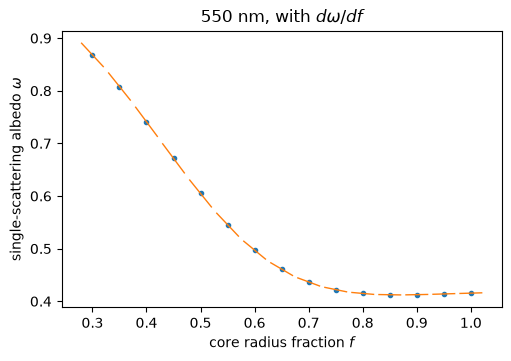
The albedo across core fractions, with the tangent the derivative gives at each point. The albedo falls as the core grows, to a shallow minimum near \(f = 0.87\), where the shell is thin and the lensing it gave is mostly gone:

fractions = np.linspace(0.3, 1.0, 15)
ssa, slope = [], []
for frac in fractions:
    p = scatrs.LayeredSphere.coated(bc, sulfate, core_fraction=frac)
    e = scatrs.Ensemble(p, coated.size).compute(0.55, derivatives=["layer0.radius_fraction"])
    ssa.append(float(e.ssa))
    slope.append(float(e.d("layer0.radius_fraction").ssa))
ssa, slope = np.array(ssa), np.array(slope)

fig, ax = plt.subplots(figsize=(5, 3.5), layout="constrained")
ax.plot(fractions, ssa, "o", ms=3)
for fr, s, ds in zip(fractions, ssa, slope, strict=True):
    dx = np.array([-0.02, 0.02])
    ax.plot(fr + dx, s + ds * dx, color="C1", lw=1)
ax.set(xlabel="core radius fraction $f$", ylabel="single-scattering albedo $\\omega$",
       title="550 nm, with $d\\omega/df$")
plt.show()
assert np.all(np.sign(slope[:-3]) == -1) and slope[-1] > 0

The derivatives are validated for outer size parameters up to 1000 (Limitations and known issues); the values, up to \(10^4\).