Internal validation

Every output of scatrs.mie has a declared accuracy, and the tests check it across the whole validated domain (How scatrs is validated explains why). This page shows what that accuracy is, how it is checked, and how much margin the checks leave. The averages over size distributions have error estimates instead, which are checked at the end of the page.

The declared accuracy

Inside the validated domain (\(10^{-6} \le x \le 2\cdot10^4\), \(0 < \mathrm{Re}\,m \le 10\), \(0 \le \mathrm{Im}\,m \le 10\), \(\lvert m\rvert \ge 0.1\)), every output is within

\[C\,(\kappa' + \mathrm{cond})\,2^{-52}\]

of the exact value, where \(2^{-52} \approx 2.2\cdot10^{-16}\) is the precision of a double:

• cond is the output’s condition number, how much it changes, relative to its size, when \(x\) and \(m\) change by a relative amount. Rounding the inputs to double precision alone moves the output by up to about \(\mathrm{cond}\cdot2^{-53}\), so no method can do better. It is large next to the sharp resonances of weakly absorbing spheres.

• κ′ grows with the size of the sphere, roughly like \(\lvert m\rvert x\): the number of terms of the series, and the cancellation between them, grow with it.

• C is a constant for each kind of output, set at least four times the worst error found anywhere in the tests (16 for the efficiencies and \(g\), for example).

The error is measured relative to the output (for amplitudes and phase-matrix elements, relative to their typical size, so that deep minima of the angular pattern are not held to a relative standard they cannot meet). Homogeneous spheres (Lorenz–Mie) gives the exact definitions.

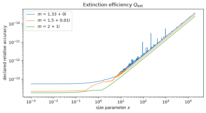
In practice the declared accuracy of the extinction efficiency runs from about \(10^{-14}\) for small spheres to a few times \(10^{-10}\) for the largest, with spikes at the resonances of non-absorbing spheres, where the output itself is that sensitive to the inputs:

import json
from pathlib import Path

import matplotlib.pyplot as plt
import numpy as np

from scatrs import mie

xs = np.geomspace(1e-3, 2e4, 3000)
fig, ax = plt.subplots(figsize=(7, 3.8), layout="constrained")
for m in (1.33 + 0j, 1.5 + 0.01j, 2 + 1j):
    q = mie.efficiencies(xs, m, derivatives=True)
    d = {p: q.d(p).q_ext for p in ("x", "m_real", "m_imag")}
    cond = (xs * abs(d["x"]) + abs(m.real) * abs(d["m_real"]) + abs(m.imag) * abs(d["m_imag"]))
    cond /= q.q_ext
    kappa = (1 + max(1, abs(m)) * xs) * max(1, abs(m) / abs(m - 1))
    declared = 16 * (kappa + cond) * 2.0**-52
    ax.loglog(xs, declared, lw=1, label=f"$m$ = {m.real:g} + {m.imag:g}i")
    assert declared.max() < 1e-8
ax.set(xlabel="size parameter $x$", ylabel="declared relative accuracy",
       title="Extinction efficiency $Q_\\mathrm{ext}$")
ax.legend()
plt.show()

How it is checked

Two tests enforce the declared accuracy, on Linux, macOS and Windows, for every change:

• Against Arb. scatrs/tests/mie_reference.rs compares every output with reference values computed independently in Arb ball arithmetic, with rigorous error bounds (Reference suite): 306 spheres for the values, 80 for the derivatives, at size parameters from \(10^{-6}\) to \(2\cdot10^4\) and refractive indices from near 1 to metal-like.

• On a dense grid. scatrs/tests/mie_accuracy_map.rs compares the double-precision results with the same computation in double-double arithmetic (about 32 digits, itself checked against Arb) on a grid of 104 size parameters from \(10^{-6}\) to \(2\cdot10^4\) against 28 refractive indices, with the amplitudes at 41 angles.

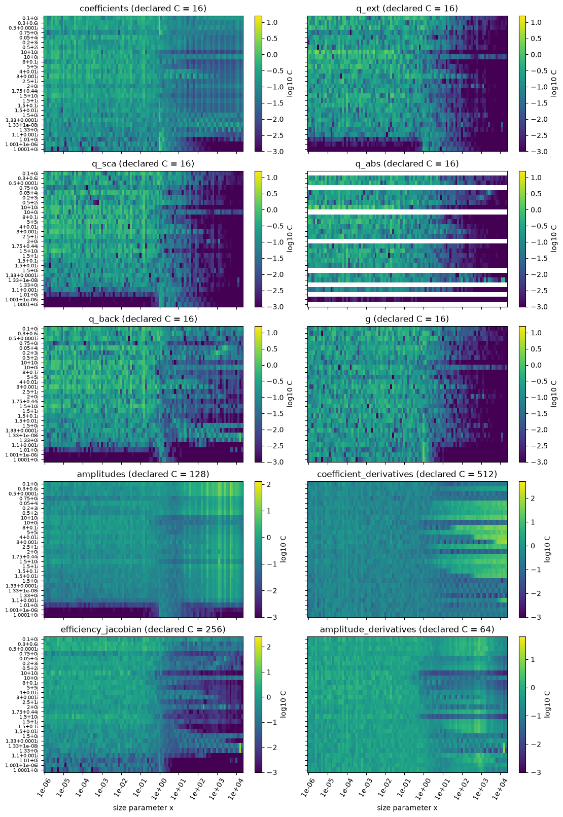
The maps below show the result of the second test. Each cell is the constant \(C\) that the worst error at that point would need,

\[C = \frac{\text{error}}{(\kappa' + \mathrm{cond})\,2^{-52}},\]

so a cell below the declared constant passes, and the colour scale ends at the declared constant. The table gives the worst value of each map against its declared constant.

def load(name):
    """An accuracy map: its size parameters, refractive indices and output names."""
    data = json.loads(Path("data", name).read_text())
    return data, np.array(data["x"]), [complex(*p) for p in data["m"]], list(data["c"])


def worst_c(data, names):
    """Print the worst C of each output against its declared constant; check the margin of 4."""
    print(f"{'output':<26}{'worst C':>10}{'declared':>10}")
    for name in names:
        # null (a non-finite C) becomes NaN, which fails the check below.
        worst = np.max(np.array(data["c"][name], dtype=float))
        print(f"{name:<26}{worst:10.2f}{data['declared'][name]:10.0f}")
        assert 4 * worst <= data["declared"][name], f"{name}: margin below 4"


def plot_map(data, x, m, names, rows, height):
    """log10 C of each output: size parameter across, refractive index down."""
    fig, axes = plt.subplots(
        rows, 2, figsize=(11, height), sharex=True, sharey=True, layout="constrained"
    )
    labels = [f"{z.real:g}{z.imag:+g}i" for z in m]
    for ax, name in zip(axes.flat, names, strict=True):
        c = np.array(data["c"][name], dtype=float).T
        with np.errstate(divide="ignore"):
            image = ax.pcolormesh(
                np.arange(len(x) + 1), np.arange(len(m) + 1), np.log10(c),
                vmin=-3, vmax=np.log10(data["declared"][name]), cmap="viridis",
            )
        ax.set_title(f"{name} (declared C = {data['declared'][name]:g})")
        fig.colorbar(image, ax=ax, label="log10 C")
    ticks = np.arange(0, len(x), 10)
    for ax in axes[-1]:
        ax.set_xticks(ticks + 0.5, [f"{x[i]:.0e}" for i in ticks], rotation=60)
        ax.set_xlabel("size parameter x")
    for ax in axes[:, 0]:
        ax.set_yticks(np.arange(len(m)) + 0.5, labels, fontsize=7)
    plt.show()


data, x, m, names = load("mie-accuracy-map.json")
print(f"{len(x)} size parameters × {len(m)} refractive indices")
worst_c(data, names)

104 size parameters × 28 refractive indices
output                       worst C  declared
coefficients                    2.28        16
q_ext                           2.50        16
q_sca                           1.62        16
q_abs                           2.49        16
q_back                          1.68        16
g                               1.64        16
amplitudes                     18.57       128
coefficient_derivatives       108.10       512
efficiency_jacobian            39.34       256
amplitude_derivatives           8.39        64

Every output stays well inside its declared accuracy. The efficiencies and \(g\) use at most a fifth of theirs, and the amplitudes at most about a seventh, largest for refractive indices below 1 and for metal-like spheres. White cells are exact, such as \(Q_\text{abs}\) of a real refractive index, which is exactly 0.

plot_map(data, x, m, names, rows=5, height=16)

The phase matrix and the Greek coefficients

The phase matrix and the Greek coefficients follow the same model, with a term for the quadrature added to the Greek coefficients (The accuracy model). Two more tests enforce them:

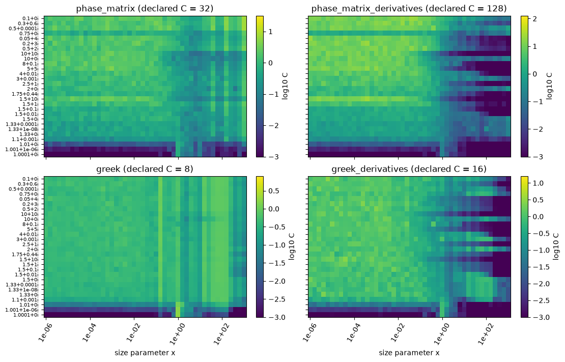
• scatrs/tests/mie_greek_reference.rs compares them with the Arb reference values: 18 cases (17 spheres, one at two orders) from \(x = 0.1\) to 200, where the worst \(C\) is 0.59 for the phase matrix and 0.61 for the Greek coefficients.

• scatrs/tests/mie_greek_accuracy_map.rs compares them with double-double on a grid of 46 size parameters from \(10^{-6}\) to \(10^3\) against the 28 refractive indices of the Mie map, with the normalized phase matrix at 13 cosines (through the forward peak, the sides and the glory) and the Greek coefficients up to all orders for \(x \le 160\) and to order 100 above, each with its derivatives.

The double-double Greek coefficients are slow for large spheres, so the map stops at \(x = 10^3\). A weekly test checks larger spheres: at \(x = 2\cdot10^3\) up to all orders (\(m = 1.33\) and \(0.3 + 0.6i\)), and at \(x = 10^4\) (\(m = 1.5 + 0.01i\)) and \(2\cdot10^4\) (\(m = 1.33\)) up to order 64. Its worst \(C\) is 2.7 for the phase matrix (at \(x = 2\cdot10^3\), \(m = 0.3 + 0.6i\)) and 0.22 for the Greek coefficients (at \(x = 2\cdot10^4\)). With the quadrature term, \(C\) is at most 1.7 for the Greek coefficients everywhere it was measured.

greek, gx, gm, gnames = load("greek-accuracy-map.json")
print(f"{len(gx)} size parameters × {len(gm)} refractive indices")
worst_c(greek, gnames)

46 size parameters × 28 refractive indices
output                       worst C  declared
phase_matrix                    7.45        32
phase_matrix_derivatives       21.99       128
greek                           1.72         8
greek_derivatives               2.83        16

plot_map(greek, gx, gm, gnames, rows=2, height=7)

Layered spheres

The outputs of scatrs.layered follow the same model (Layered spheres), with the condition numbers summed over every layer’s parameters and their own constants. Inside their validated domain (\(10^{-6} \le x_L \le 10^4\) with \(|m_l|\,x_L \le 3\cdot10^4\), every index in the sphere’s domain, at most 16 layers; the derivatives up to \(x_L = 1000\)), four tests enforce them:

• scatrs/tests/layered_reference.rs compares every output with the Arb reference values, computed without scatrs’s algorithm by matching the fields at each interface directly (Reference suite): 362 particles in the domain, from \(x_L = 10^{-6}\) to \(10^4\), including thin and thick shells, absorbing cores in clear shells, metallic shells, near-unity and high-contrast indices, air shells, and up to ten layers; and the derivatives for 8 particles. The 8 reference particles outside the domain must be refused.

• scatrs/tests/layered_accuracy_map.rs compares the double-precision results with double-double on 101 outer size parameters from \(10^{-6}\) to \(10^4\) against 51 particles: 12 pairs of core and shell indices at core radius fractions \(10^{-3}\), 0.3, 0.9 and 0.999, and three- and ten-layer particles.

• scatrs/tests/layered_greek_accuracy_map.rs does the same for the phase matrix and the Greek coefficients, on 46 outer size parameters up to \(10^3\) against 21 particles.

• scatrs/tests/layered.rs checks the identities that need no reference: one layer, and layers of one index, are bitwise the homogeneous sphere; a shell of zero thickness changes nothing; an air shell gives the bare core; the Rayleigh limit; and the derivatives against central differences.

The worst \(C\) of each map against its declared constant, and the worst \(C\) over all particles at each size (empty above \(x_L = 1000\) for the derivatives):

def worst_layered(name):
    """Print the worst C of each output of a layered map; check the margin of 4."""
    data = json.loads(Path("data", name).read_text())
    print(f"{len(data['x'])} outer size parameters × {len(data['particles'])} particles")
    print(f"{'output':<26}{'worst C':>10}{'declared':>10}")
    for output, rows in data["c"].items():
        # null: outside the (derivatives') domain.
        c = np.array(rows, dtype=float)
        worst = np.nanmax(c)
        print(f"{output:<26}{worst:10.2f}{data['declared'][output]:10.0f}")
        assert 4 * worst <= data["declared"][output], f"{output}: margin below 4"
    return data


layered_map = worst_layered("layered-accuracy-map.json")
layered_greek = worst_layered("layered-greek-accuracy-map.json")

101 outer size parameters × 51 particles
output                       worst C  declared
coefficients                    5.86        32
q_ext                           6.54        32
q_sca                           2.68        16
q_abs                          37.84       256
q_back                         12.61        64
g                               2.46        16
amplitudes                     12.33       128
coefficient_derivatives        22.14      1024
efficiency_jacobian            48.44       256
amplitude_derivatives         162.90      1024
46 outer size parameters × 21 particles
output                       worst C  declared
phase_matrix                    8.80        64
greek                           2.35        16
phase_matrix_derivatives       57.68       256
greek_derivatives              48.20       256

fig, axes = plt.subplots(1, 2, figsize=(11, 4), sharey=True, layout="constrained")
for ax, data, title in [
    (axes[0], layered_map, "coefficients, efficiencies, amplitudes"),
    (axes[1], layered_greek, "phase matrix, Greek coefficients"),
]:
    x = np.array(data["x"])
    for output, rows in data["c"].items():
        c = np.array(rows, dtype=float)
        with np.errstate(all="ignore"):
            worst = np.nanmax(np.where(np.isnan(c), -np.inf, c), axis=1)
        worst[~np.isfinite(worst)] = np.nan
        ax.loglog(x, worst, lw=1, label=output)
    ax.set(xlabel="outer size parameter $x_L$", title=title)
axes[0].set_ylabel("worst $C$ over the particles")
for ax in axes:
    ax.legend(fontsize=7)
plt.show()

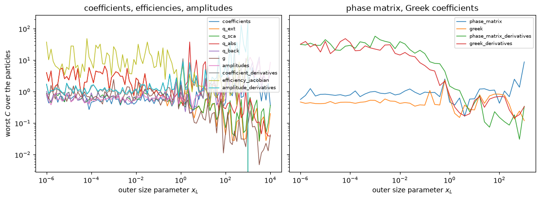
The values use at most a quarter of their constants anywhere, and so do the derivatives up to \(x_L = 1000\). Above it, the amplitude derivatives of thin lossless shells grow with the particle: for an air shell of a thousandth of the radius, the forward amplitude’s derivative with respect to the shell’s index would exceed its constant by 1.7 times at \(x_L = 10^4\). The rounding errors of the recurrences at the shell’s two surfaces are alike from one order to the next, so they add up in the forward sum, and the derivatives’ domain ends at 1000.

Spheroids

The outputs of scatrs.tmatrix are converged to a tolerance rtol and come with an error estimate \(\hat\varepsilon\) (Spheroids). Inside the validated domain (aspect ratios from 1/5 to 5, equal-volume \(x \ge 10^{-6}\), \(|m|\,x_{\max} \le 60\) with \(x_{\max}\) the size parameter of the longest semi-axis, \(1.3 \le \mathrm{Re}\,m \le 3\), \(\mathrm{Im}\,m \le 0.5\)), every output is within \(C\cdot\max(\mathtt{rtol}, \hat\varepsilon)\) of the exact value, in the measures of the sphere’s outputs (\(Q_{\mathrm{abs}}\) relative to \(Q_{\mathrm{ext}}\), the Greek coefficients relative to the largest \(|\alpha_1|\), the phase matrix relative to \(\max(F_{11}, 1)\), normalized). Three tests enforce it:

• scatrs/tests/spheroid_reference.rs compares with Arb reference values of an EBCM computed from its definition, with no simplification of the integrands (Reference suite), for 10 spheroids. At a fixed truncation, the efficiencies and the T-matrix elements must be within 4 times the solution’s own estimate on each of the three precision paths (f64, refined and double-double); the converged efficiencies must be within the declared tolerance.

• scatrs/tests/spheroid_published.rs compares with the arbitrary-precision \(Q_\text{sca}\) and \(Q_\text{ext}\) published by Somerville, Auguié & Le Ru (2013) for two spheroids inside the domain, one of them the benchmark of Kuik, de Haan & Hovenier (1992) (External validation).

• scatrs/tests/tmatrix_accuracy_map.rs compares the default results (rtol = 1e-8) with a reference using more orders and nodes and every mode refined, for 349 spheroids: 8 aspect ratios, \(x\) from \(10^{-6}\) to 14 and four indices, up to \(|m|\,x_{\max} = 70\).

The worst ratio of each error to \(\max(\mathtt{rtol}, \hat\varepsilon)\) inside the domain, against the declared constant:

data = json.loads(Path("data", "spheroid-accuracy-map.json").read_text())
points = data["points"]
ratios = np.array([p["ratios"] for p in points])
inside = np.array([p["inside"] for p in points])
print(f"{len(points)} spheroids, {inside.sum()} inside the domain")
print(f"{'output':<10}{'worst inside':>14}{'worst outside':>15}{'declared C':>12}")
for k, output in enumerate(data["outputs"]):
    worst_in, worst_out = ratios[inside, k].max(), ratios[~inside, k].max()
    print(f"{output:<10}{worst_in:14.3f}{worst_out:15.3f}{data['declared'][output]:12.0f}")
    assert 4 * worst_in <= data["declared"][output], f"{output}: margin below 4"

349 spheroids, 347 inside the domain
output      worst inside  worst outside  declared C
q_ext              0.029          0.001           4
q_sca              0.022          0.001           4
q_abs              0.033          0.000          16
g                  0.014          0.000           4
q_back             1.040          0.008          16
greek              0.569          0.002          16
phase              0.102          0.002          16

fig, ax = plt.subplots(figsize=(7, 4), layout="constrained")
phase = np.array([p["phase"] for p in points])
for k, output in enumerate(data["outputs"]):
    ax.semilogy(phase, np.maximum(ratios[:, k], 1e-12), ".", ms=4, label=output)
ax.axvline(60, color="k", lw=0.8, ls="--")
ax.set(
    xlabel=r"$|m|\,x_{\max}$",
    ylabel=r"error / max(rtol, estimate)",
    ylim=(1e-8, 10),
)
ax.legend(fontsize=7, ncols=2)
plt.show()

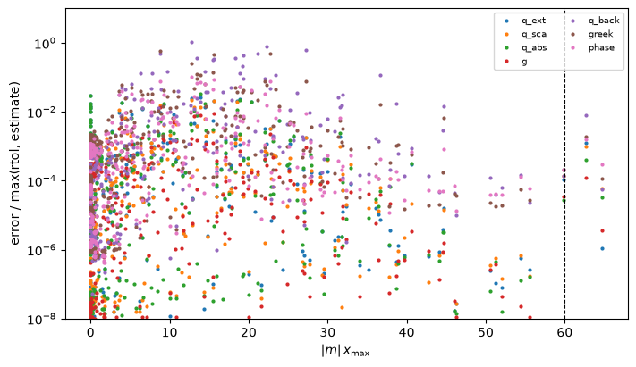
The estimates are conservative: the cross sections and \(g\) stay below a twentieth of \(\max(\mathtt{rtol}, \hat\varepsilon)\), and only \(Q_{\mathrm{back}}\) reaches it (1.04 times, at \(\varepsilon = 1/3\), \(x = 4\)), well within its constant. Past \(|m|\,x_{\max} = 60\) the results are as accurate, but the modes that need refinement make one spheroid cost minutes, so the domain ends there.

Ensembles

The averages over size distributions (Ensembles) add the error of the size integration and of the cut-offs of the distribution. Every output has an estimate of that error (result.error), and the integration is refined until the estimates of the cross sections, \(g\) and the moments meet the tolerance rtol (default \(10^{-6}\)). The Mie solutions’ own errors, declared above, are far smaller at the tolerances the ensembles accept, and are not included. A spheroid’s are: every size node adds its declared error, its constant times \(\max(\tau, \hat\varepsilon)\) for its own estimate and the node tolerance \(\tau\) (Spheroids: the direct path).

The test error_estimates_bound_the_true_errors in scatrs/tests/ensemble.rs checks the estimates for every change. It computes nine distributions of spheres and two of layered spheres at rtol \(10^{-6}\) and again at rtol \(10^{-11}\) (the reference), with backscattering refined, the Greek coefficients to order 24, the phase matrix at \(\mu = 1, 0.7, 0, -1\), and the derivatives with respect to every parameter of the distribution and of the particle (\(\mathrm{Re}\,m\) and \(\mathrm{Im}\,m\) of every layer, and the radius fractions):

Distribution	\(m\)	\(\lambda\)
lognormal, \(r_g = 0.08\), \(\sigma_g = 1.6\)	\(1.43 + 10^{-8}i\)	0.5
lognormal, \(r_g = 5\), \(\sigma_g = 1.3\)	\(1.5 + 0.01i\)	0.5
lognormal, \(r_g = 0.001\), \(\sigma_g = 2\)	\(1.5\)	0.5
lognormal, \(r_g = 0.5\), \(\sigma_g = 1.05\)	\(1.33 + 10^{-3}i\)	0.6
gamma, \(a = 2\), \(b = 0.1\)	\(1.33 + 10^{-3}i\)	0.65
modified gamma, \(\alpha = 2\), \(b = 15\), \(\gamma = 0.5\)	\(1.5 + 10^{-3}i\)	0.5
power law, \(\alpha = 3.5\) on \([0.01, 5]\)	\(1.5 + 0.01i\)	0.5
tabulated, \((0.05, 0.1, 0.4, 1)\), densities \((0, 3, 1, 0.2)\)	\(2 + 0.5i\)	0.4
multimodal: weight 1000, lognormal \(r_g = 0.05\), \(\sigma_g = 1.5\); weight 1, lognormal \(r_g = 1\), \(\sigma_g = 1.4\)	\(1.53 + 0.005i\)	0.55
lognormal, \(r_g = 0.1\), \(\sigma_g = 1.6\), coated (core fraction 0.6)	core \(1.95 + 0.79i\), shell \(1.43 + 10^{-8}i\)	0.55
gamma, \(a = 0.8\), \(b = 0.1\), three layers (fractions 0.3, 0.8)	\(1.6 + 0.3i\), \(2 + 0.05i\), \(1.33 + 10^{-6}i\)	0.5

Both results must converge, and the refined cross sections must be within rtol of the reference (\(g\) within \(2\cdot10^{-6}\)). The true errors of the refined outputs (\(\langle C_\text{ext}\rangle\), \(\langle C_\text{sca}\rangle\), \(\langle C_\text{back}\rangle\), \(g\) and the moments) must be within their estimates, and those of the other outputs (the other values, the Greek coefficients, the phase matrix and every derivative) within 2 times their estimates. The worst ratio of true error to estimate is 0.003 for the refined outputs and 1.210 for the others. Example: an aerosol size distribution shows the same comparison for one distribution.

For spheroids, scatrs/tests/ensemble_spheroid.rs checks the same: a lognormal of prolate spheroids (\(a/c = 1/3\), \(r_g = 0.03\), \(\sigma_g = 1.4\), \(m = 1.53 + 0.008i\), \(\lambda = 1\)) at rtol \(10^{-6}\) against rtol \(10^{-10}\), with backscattering refined, the Greek coefficients to order 8 and the phase matrix at three cosines. Every scalar output is within its estimate, which the nodes’ declared errors make 10 to 1000 times the true error, and the Greek coefficients and the phase matrix within twice theirs. The same file checks that an aspect ratio of 1 is the sphere ensemble within the estimates, that a monodisperse ensemble is the single spheroid, and the Jacobians (the aspect ratio, \(\mathrm{Re}\,m\), \(\mathrm{Im}\,m\), the distribution’s parameters, a monodisperse radius and a mixture’s spheroid component) against central differences.

What that supports:

• The refined outputs. When converged is true, their estimates meet rtol, and on the test grid they bounded the true errors with a wide margin. The estimates of ratios (\(\omega\), \(g\), the lidar ratio, \(r_\text{eff}\) and the normalized outputs) are propagated from those of their numerator and denominator.

• The other outputs are integrated on the size panels that the refined outputs chose, so their estimates are only as good as those panels are for them. On the grid their true errors reached 1.21 times their estimates. This includes \(\langle C_\text{abs}\rangle\), which is refined only to rtol of \(\langle C_\text{ext}\rangle\).

• Backscattering is indicative unless refined. Without refine_backscatter=True, the estimates of \(\langle C_\text{back}\rangle\) and the lidar ratio come from panels that may not resolve the narrow glory ripples, and the true errors can exceed them.

Two cases are flagged with converged = false rather than estimated well:

• Non-absorbing spheres. Without absorption, the efficiencies of large spheres have narrow resonance ripples, which can take more than max_panels panels to resolve. For a lognormal with \(r_g = 1\), \(\sigma_g = 2\) and \(m = 1.33\) at \(\lambda = 0.5\), the integration stops at 4096 panels with an estimate of about \(10^{-5}\) of \(\langle C_\text{ext}\rangle\); the true error of the stopped result is \(1.0\cdot10^{-6}\). With max_panels raised it converges at 5020 panels, but its true error, \(1.1\cdot10^{-6}\) of \(\langle C_\text{ext}\rangle\), exceeds its estimate, \(9.7\cdot10^{-7}\).

• Derivatives with respect to \(\mathrm{Im}\,m\) at \(\mathrm{Im}\,m = 0\) have a spike at every resonance and do not converge; the values do.