Example: an aerosol size distribution

An Ensemble averages the optical properties of spheres over a size distribution, at many wavelengths, with an error estimate for every output and, on request, derivatives. See Ensembles for the method. This page runs whenever the documentation is built; its checks are asserts, so a failing check fails the build.

A sulfate aerosol across the spectrum

A lognormal distribution of sulfate-like droplets: median radius \(r_g = 0.08\) µm, width \(\sigma_g = 1.6\), refractive index \(m = 1.43 + 10^{-8}i\) at every wavelength. Radii and wavelengths share a unit (µm here), so the cross sections are in µm² per particle.

import matplotlib.pyplot as plt
import numpy as np

import scatrs

m = 1.43 + 1e-8j
sulfate = scatrs.Ensemble(scatrs.Sphere(m), scatrs.LogNormal(median_radius=0.08, width=1.6))
wavelength = np.array([0.35, 0.40, 0.45, 0.50, 0.55, 0.67, 0.87, 1.0])
r = sulfate.compute(wavelength)
print(f"{'λ (µm)':>7}{'C_ext (µm²)':>13}{'1 - ω':>10}{'g':>8}{'panels':>8}")
for row in zip(wavelength, r.c_ext, 1 - r.ssa, r.g, r.panels, strict=True):
    print("{:7.2f}{:13.4e}{:10.1e}{:8.4f}{:8d}".format(*row))
assert r.converged.all()
assert np.all(np.diff(r.c_ext) < 0) and np.all(np.diff(r.g) < 0)
assert np.all(1 - r.ssa < 1e-6)

 λ (µm)  C_ext (µm²)     1 - ω       g  panels
   0.35   5.6498e-02   6.0e-08  0.7165      52
   0.40   4.6459e-02   6.2e-08  0.6978      42
   0.45   3.8162e-02   6.5e-08  0.6775      35
   0.50   3.1417e-02   6.9e-08  0.6561      30
   0.55   2.5967e-02   7.3e-08  0.6340      30
   0.67   1.6784e-02   8.6e-08  0.5802      28
   0.87   8.6864e-03   1.1e-07  0.4934      24
   1.00   5.9044e-03   1.4e-07  0.4419      27

Extinction falls and the scattering becomes less forward-peaked as the wavelength grows past the particles. The Ångström exponent \(-d\ln\langle C_\text{ext}\rangle/d\ln\lambda\), here from neighbouring wavelengths, rises from about 1.5 in the ultraviolet towards the Rayleigh limit of 4 as the particles become small compared with the wavelength.

angstrom = -np.diff(np.log(r.c_ext)) / np.diff(np.log(wavelength))
mid = np.sqrt(wavelength[1:] * wavelength[:-1])
for lam, a in zip(mid, angstrom, strict=True):
    print(f"λ ≈ {lam:.2f} µm: Ångström exponent {a:.2f}")
assert np.all(np.diff(angstrom) > 0) and 1 < angstrom[0] and angstrom[-1] < 4

λ ≈ 0.37 µm: Ångström exponent 1.47
λ ≈ 0.42 µm: Ångström exponent 1.67
λ ≈ 0.47 µm: Ångström exponent 1.85
λ ≈ 0.52 µm: Ångström exponent 2.00
λ ≈ 0.61 µm: Ångström exponent 2.21
λ ≈ 0.76 µm: Ångström exponent 2.52
λ ≈ 0.93 µm: Ångström exponent 2.77

The same on a fine wavelength grid, next to the distribution itself: in number most particles are far smaller than the wavelength, but the cross section weights them by area and more, so the larger ones dominate the optics.

lam = np.geomspace(0.3, 2.0, 60)
fine_grid = sulfate.compute(lam)

radius = np.geomspace(0.005, 1.5, 400)
number = np.exp(-np.log(radius / 0.08) ** 2 / (2 * np.log(1.6) ** 2))  # dN/d ln r, unnormalized
fig, (ax1, ax2, ax3) = plt.subplots(1, 3, figsize=(12, 3.5), layout="constrained")
for weight, label in [(1, "number"), (radius**2, "area"), (radius**3, "volume")]:
    density = number * weight
    ax1.semilogx(radius, density / density.max(), label=label)
ax1.axvline(fine_grid.effective_radius[0], color="0.5", ls="--", lw=0.8)
ax1.text(fine_grid.effective_radius[0] * 1.08, 0.05, "$r_\\mathrm{eff}$", color="0.4")
ax1.set(xlabel="radius (µm)", ylabel="d/d ln r (scaled to 1)", title="Distribution")
ax1.legend()
ax2.loglog(lam, fine_grid.c_ext)
ax2.loglog(lam, fine_grid.c_ext[-1] * (lam / lam[-1]) ** -4, ":", color="0.5", label="$\\lambda^{-4}$")
ax2.set(xlabel="wavelength (µm)", ylabel="$\\langle C_\\mathrm{ext}\\rangle$ (µm²)", title="Extinction")
ax2.legend()
ax3.semilogx(lam, fine_grid.g)
ax3.set(xlabel="wavelength (µm)", ylabel="$g$", title="Asymmetry parameter")
for ax in (ax2, ax3):
    ax.set_xticks([0.3, 0.5, 1, 2], ["0.3", "0.5", "1", "2"], minor=False)
    ax.set_xticks([], minor=True)
plt.show()
assert fine_grid.converged.all()

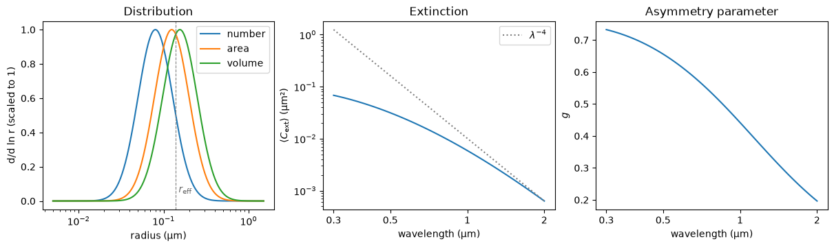
The moments do not depend on the wavelength. The effective radius of a lognormal is \(r_g\exp\bigl(\tfrac52\ln^2\sigma_g\bigr)\); the integrated one, over the cut-off range, agrees with it within its error estimate, which includes the cut-offs.

closed_form = 0.08 * np.exp(2.5 * np.log(1.6) ** 2)
print(f"r_eff = {r.effective_radius[0]:.10f} µm, closed form {closed_form:.10f} µm, "
      f"estimate {r.error.effective_radius[0]:.1e} µm")
assert np.all(abs(r.effective_radius - closed_form) <= r.error.effective_radius)

r_eff = 0.1389737635 µm, closed form 0.1389737635 µm, estimate 5.6e-08 µm

Error estimates and convergence

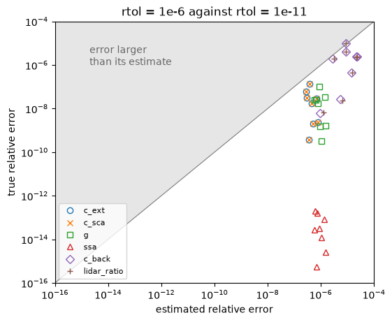
Every output has an error estimate (r.error), and r.converged says whether every refined quantity met the tolerance rtol (default \(10^{-6}\)) within max_panels panels. Here the default result is compared with one at rtol=1e-11: the true errors of the refined outputs are within rtol and within their estimates. The backscattering is not refined by default, so its estimate is only indicative (Ensembles); refine_backscatter=True refines it too.

tight = sulfate.compute(wavelength, rtol=1e-11, max_panels=50_000)
print(f"{'output':<10}{'largest error/estimate':>24}{'largest relative error':>24}")
for name in ("c_ext", "c_sca", "g", "ssa", "c_back", "lidar_ratio"):
    value, exact, estimate = getattr(r, name), getattr(tight, name), getattr(r.error, name)
    error = abs(value - exact)
    print(f"{name:<10}{np.max(error / estimate):24.2e}{np.max(error / abs(exact)):24.2e}")
    if name in ("c_ext", "c_sca", "g", "ssa"):
        assert np.all(error <= estimate)
    if name in ("c_ext", "c_sca"):
        assert np.all(error <= 1e-6 * exact)

output      largest error/estimate  largest relative error
c_ext                     3.59e-01                1.32e-07
c_sca                     3.59e-01                1.32e-07
g                         1.20e-01                1.04e-07
ssa                       3.38e-07                2.06e-13
c_back                    1.14e+00                9.85e-06
lidar_ratio                1.07e+00                9.72e-06

Each point below is one output at one wavelength. The refined outputs lie far below the diagonal: their estimates are conservative. The backscattering, not refined, can lie above it.

fig, ax = plt.subplots(figsize=(5.5, 4.5), layout="constrained")
markers = {"c_ext": "o", "c_sca": "x", "g": "s", "ssa": "^", "c_back": "D", "lidar_ratio": "+"}
for name, marker in markers.items():
    value, exact, estimate = getattr(r, name), getattr(tight, name), getattr(r.error, name)
    ax.loglog(estimate / abs(exact), abs(value - exact) / abs(exact), marker, ms=6,
              mfc="none" if marker in "osD^" else None, label=name)
lims = np.array([1e-16, 1e-4])
ax.loglog(lims, lims, color="0.5", lw=0.8)
ax.fill_between(lims, lims, 1, color="0.9", zorder=0)
ax.text(2e-15, 1e-6, "error larger\nthan its estimate", color="0.4")
ax.set(xlim=lims, ylim=lims, xlabel="estimated relative error",
       ylabel="true relative error", title="rtol = 1e-6 against rtol = 1e-11")
ax.legend(fontsize=8, loc="lower left")
plt.show()

Greek coefficients

greek= asks for the Greek coefficients of the averaged phase matrix, here to order 32, the first few at 0.55 µm. Normalized, \(\alpha_1^0 = 1\) and \(\alpha_1^1 = 3g\), with \(g\) from the asymmetry parameters of the spheres.

g = sulfate.compute(0.55, greek=32)
names = ("alpha1", "alpha2", "alpha3", "alpha4", "beta1", "beta2")
print(f"{'l':>3}" + "".join(f"{name:>11}" for name in names))
for l in range(6):
    print(f"{l:3d}" + "".join(f"{getattr(g.greek, name)[l]:11.5f}" for name in names))
print("3g =", 3 * g.g)
assert g.greek.alpha1[0] == 1
assert abs(g.greek.alpha1[1] - 3 * g.g) < 1e-13 * 3 * g.g

  l     alpha1     alpha2     alpha3     alpha4      beta1      beta2
  0    1.00000    0.00000    0.00000    0.85536    0.00000    0.00000
  1    1.90210    0.00000    0.00000    2.05030    0.00000    0.00000
  2    1.89458    3.69101    3.32088    1.86120   -0.31534    0.08008
  3    1.33455    2.02721    1.97376    1.38449   -0.21840    0.20488
  4    0.85537    1.25801    1.16393    0.83568   -0.11109    0.11463
  5    0.49121    0.63592    0.61685    0.50027   -0.07088    0.10130
3g = 1.9020994624191299

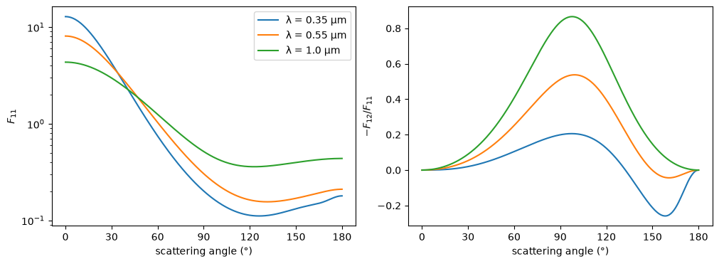
mu= asks for the averaged phase matrix at given cosines instead. Here it is at three wavelengths: the larger the particles are relative to the wavelength, the more the scattering is forward-peaked.

angles = np.linspace(0, 180, 361)
mu = np.cos(np.radians(angles))
pm = sulfate.compute([0.35, 0.55, 1.0], mu=mu)
fig, (ax1, ax2) = plt.subplots(1, 2, figsize=(10, 3.6), layout="constrained")
for i, lam in enumerate([0.35, 0.55, 1.0]):
    ax1.semilogy(angles, pm.phase.f11[i], label=f"λ = {lam} µm")
    ax2.plot(angles, -pm.phase.f12[i] / pm.phase.f11[i])
ax1.set(xlabel="scattering angle (°)", ylabel="$F_{11}$", xticks=range(0, 181, 30))
ax2.set(xlabel="scattering angle (°)", ylabel="$-F_{12}/F_{11}$", xticks=range(0, 181, 30))
ax1.legend()
plt.show()
# The phase function is normalized: ½∫F11 dμ = 1 (trapezoidal rule on this grid).
assert np.allclose(-0.5 * np.trapezoid(pm.phase.f11, mu, axis=-1), 1, rtol=1e-3)

Their error estimates are bounds, given the estimates of the tables they are projected from. Every node of a size panel fills the tables of the panel’s projector band, so the tables are smooth within a panel and the bounds are about as tight as the other estimates (Ensembles). Unnormalized (normalized=False), \(\alpha_1^0\) is \(\langle C_\text{sca}\rangle\) itself, and its estimate is less than twice that of \(\langle C_\text{sca}\rangle\).

u = sulfate.compute(0.55, greek=32, normalized=False)
exact = sulfate.compute(0.55, greek=32, normalized=False, rtol=1e-11, max_panels=50_000)
print(f"alpha1[0] = {u.greek.alpha1[0]:.12e}, c_sca = {u.c_sca:.12e}")
print(f"estimates: alpha1[0] {u.error.greek.alpha1[0]:.1e}, c_sca {u.error.c_sca:.1e}; "
      f"true error {abs(u.greek.alpha1[0] - exact.greek.alpha1[0]):.1e}")
assert abs(u.greek.alpha1[0] / u.c_sca - 1) < 1e-13
assert u.error.greek.alpha1[0] < 2 * u.error.c_sca
assert np.all(abs(u.greek.alpha1 - exact.greek.alpha1) <= u.error.greek.alpha1)

alpha1[0] = 2.596744084427e-02, c_sca = 2.596744084427e-02
estimates: alpha1[0] 2.3e-08, c_sca 1.3e-08; true error 5.2e-11

Derivatives

derivatives= names the parameters to differentiate with respect to (or True for all): the distribution’s ("median_radius", "width"), "m_real" and "m_imag". r.d(name) holds the derivatives of every output, and r.d_error(name) their estimates. Here \(\partial\langle C_\text{ext}\rangle/\partial r_g\) and \(\partial g/\partial r_g\) at 0.55 µm are checked against central differences, all at rtol=1e-11 so that the integration error does not swamp the difference.

def run(median_radius, **kwargs):
    ens = scatrs.Ensemble(scatrs.Sphere(m), scatrs.LogNormal(median_radius, 1.6))
    return ens.compute(0.55, rtol=1e-11, max_panels=50_000, **kwargs)


d = run(0.08, derivatives=["median_radius"])
h = 1e-4 * 0.08
plus, minus = run(0.08 + h), run(0.08 - h)
for name in ("c_ext", "g"):
    exact = getattr(d.d("median_radius"), name)
    fd = (getattr(plus, name) - getattr(minus, name)) / (2 * h)
    print(f"d {name} / d median_radius: {exact:.10f}, central difference {fd:.10f}, "
          f"relative difference {abs(exact / fd - 1):.0e}")
    assert abs(exact - fd) < 1e-7 * abs(fd)

d c_ext / d median_radius: 1.3209486289, central difference 1.3209486330, relative difference 3e-09
d g / d median_radius: 3.0621969057, central difference 3.0621969907, relative difference 3e-08

A mixture with a coarse mode

A Mixture averages over an external mixture of ensembles, each with a weight, its relative number concentration. Here the sulfate is mixed with one coarse, weakly absorbing particle per thousand (\(r_g = 0.4\) µm, \(\sigma_g = 1.8\), \(m = 1.50 + 10^{-3}i\)). Cross sections average with the number fractions \(w_i/\sum w\); the phase matrix, and so the Greek coefficients, with \(w_i\langle C_\text{sca}\rangle_i\).

coarse = scatrs.Ensemble(scatrs.Sphere(1.50 + 1e-3j), scatrs.LogNormal(median_radius=0.4, width=1.8))
weights = (1.0, 1e-3)
mixture = scatrs.Mixture([(weights[0], sulfate), (weights[1], coarse)])
lam = np.array([0.35, 0.55, 1.0])
mix = mixture.compute(lam, greek=16, derivatives=["c1.weight"])
fine = sulfate.compute(lam, greek=16)
big = coarse.compute(lam, greek=16)
f = np.array(weights) / sum(weights)
print(f"{'λ (µm)':>7}{'C_ext (µm²)':>13}{'ω':>9}{'g':>8}{'coarse share of C_ext':>23}")
for i in range(len(lam)):
    share = f[1] * big.c_ext[i] / mix.c_ext[i]
    print(f"{lam[i]:7.2f}{mix.c_ext[i]:13.4e}{mix.ssa[i]:9.5f}{mix.g[i]:8.4f}{share:23.3f}")
c_sca = f[0] * fine.c_sca + f[1] * big.c_sca
alpha1 = (
    f[0] * fine.c_sca[:, None] * fine.greek.alpha1 + f[1] * big.c_sca[:, None] * big.greek.alpha1
) / c_sca[:, None]
assert np.allclose(mix.c_ext, f[0] * fine.c_ext + f[1] * big.c_ext, rtol=1e-13, atol=0)
assert np.allclose(mix.ssa, c_sca / mix.c_ext, rtol=1e-13, atol=0)
assert np.allclose(mix.greek.alpha1, alpha1, rtol=0, atol=1e-13)
assert mix.converged.all()

 λ (µm)  C_ext (µm²)        ω       g  coarse share of C_ext
   0.35   5.8843e-02  0.99866  0.7170                  0.041
   0.55   2.8565e-02  0.99808  0.6399                  0.092
   1.00   8.8198e-03  0.99644  0.5246                  0.331

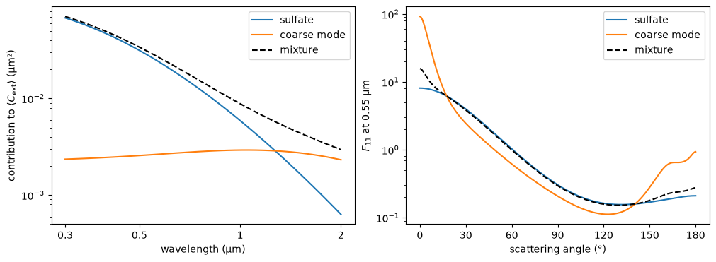
Across the spectrum the coarse mode takes over the extinction as the wavelength grows, and at 0.55 µm it already sharpens the forward peak of the phase function.

lam = np.geomspace(0.3, 2.0, 40)
mix_l = mixture.compute(lam)
fine_l = sulfate.compute(lam)
coarse_l = coarse.compute(lam)
at_550 = dict(mu=mu)
phases = {
    "sulfate": sulfate.compute(0.55, **at_550).phase.f11,
    "coarse mode": coarse.compute(0.55, **at_550).phase.f11,
    "mixture": mixture.compute(0.55, **at_550).phase.f11,
}

fig, (ax1, ax2) = plt.subplots(1, 2, figsize=(10, 3.6), layout="constrained")
ax1.loglog(lam, f[0] * fine_l.c_ext, label="sulfate")
ax1.loglog(lam, f[1] * coarse_l.c_ext, label="coarse mode")
ax1.loglog(lam, mix_l.c_ext, "k--", label="mixture")
ax1.set(xlabel="wavelength (µm)", ylabel="contribution to $\\langle C_\\mathrm{ext}\\rangle$ (µm²)")
ax1.set_xticks([0.3, 0.5, 1, 2], ["0.3", "0.5", "1", "2"], minor=False)
ax1.set_xticks([], minor=True)
ax1.legend()
for label, f11 in phases.items():
    ax2.semilogy(angles, f11, "k--" if label == "mixture" else "-", label=label)
ax2.set(xlabel="scattering angle (°)", ylabel="$F_{11}$ at 0.55 µm", xticks=range(0, 181, 30))
ax2.legend()
plt.show()
assert np.allclose(mix_l.c_ext, f[0] * fine_l.c_ext + f[1] * coarse_l.c_ext, rtol=1e-13, atol=0)

The derivative with respect to a weight follows from the number fractions: \(\partial\langle C_\text{ext}\rangle/\partial w_1 = (\langle C_\text{ext}\rangle_1 - \langle C_\text{ext}\rangle)/\sum w\), where \(\langle C_\text{ext}\rangle_1\) is the coarse mode’s. The coarse particles dominate it: per unit of \(w_1\), \(\langle C_\text{ext}\rangle\) changes by about 40 to 330 times its value.

dw = mix.d("c1.weight").c_ext
print("d C_ext / d c1.weight:", dw, "relative to C_ext:", dw / mix.c_ext)
assert np.all((dw / mix.c_ext > 39) & (dw / mix.c_ext < 340))
assert np.allclose(dw, (big.c_ext - mix.c_ext) / sum(weights), rtol=1e-12, atol=0)

d C_ext / d c1.weight: [2.34285153 2.59469046 2.91253492] relative to C_ext: [ 39.81549411  90.83546918 330.22633359]

An optics table

Distribution parameters given as arrays make a grid of distributions, as an optics table needs; they broadcast together like NumPy arrays, and the results have the grid’s axes before the wavelengths’. The grid’s distributions share their size nodes, so the whole table costs little more than its broadest distribution alone (Ensembles). Here, sulfate lognormals over 12 median radii and 3 widths at four wavelengths.

radii, widths = np.geomspace(0.02, 0.5, 12), np.array([1.4, 1.6, 1.8])
table = scatrs.Ensemble(scatrs.Sphere(m), scatrs.LogNormal(radii[:, None], widths))
t = table.compute([0.35, 0.55, 0.87, 1.6], greek=16)
print(t)

fig, ax = plt.subplots(figsize=(5.5, 3.8), layout="constrained")
for j, width in enumerate(widths):
    ax.loglog(radii, t.c_ext[:, j, 1] / (np.pi * t.grid["median_radius"][:, j] ** 2),
              label=f"$\\sigma_g$ = {width}")
ax.set(xlabel="median radius $r_g$ (µm)", ylabel="$\\langle C_\\mathrm{ext}\\rangle/(\\pi r_g^2)$ at 0.55 µm")
ax.legend()
plt.show()
assert t.c_ext.shape == (12, 3, 4) and t.greek.alpha1.shape == (12, 3, 4, 17)
assert t.converged.all()

EnsembleResult(shape=(12, 3, 4), greek=(12, 3, 4, 17), params=(), grid=('median_radius', 'width'), converged=144/144)

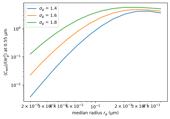
Each point of the grid meets its own tolerance and differs from its own ensemble within the error estimates. A grid computes values only: derivatives come from an ensemble of one distribution.

one = scatrs.Ensemble(scatrs.Sphere(m), scatrs.LogNormal(radii[5], widths[1])).compute([0.35, 0.55, 0.87, 1.6])
assert np.all(abs(t.c_ext[5, 1] - one.c_ext) <= 2 * (t.error.c_ext[5, 1] + one.error.c_ext))

Distributions that are not one family’s parameters, such as measured size distributions, go in a list instead, of any kinds; they share their size nodes in the same way, and the results have one axis for the list.

measured = [
    scatrs.Tabulated([0.02, 0.08, 0.2, 0.5], [0.0, 3.0, 1.0, 0.0]),
    scatrs.Tabulated([0.05, 0.1, 0.3, 0.8], [0.0, 2.0, 1.5, 0.0]),
    scatrs.LogNormal(0.08, 1.6),
]
batch = scatrs.Ensemble(scatrs.Sphere(m), measured).compute([0.35, 0.55, 0.87, 1.6])
print(batch)
assert batch.c_ext.shape == (3, 4) and batch.converged.all()

EnsembleResult(shape=(3, 4), params=(), converged=12/12)