Example: mineral dust as spheroids

Mineral dust grains are irregular, and spheres describe their scattering poorly: they overestimate the backscattering and cannot depolarize light at all. Randomly oriented spheroids are the usual replacement in remote sensing (Dubovik et al. 2006). This page computes them with scatrs.tmatrix: the efficiencies and how little they depend on shape, the phase matrix and what shape does change, a mixture of shapes, the Greek coefficients, the convergence and precision of each result, the T-matrix itself, derivatives, and the validated domain. See Spheroids for the method. This page runs whenever the documentation is built; its checks are asserts, so a failing check fails the build.

A spheroid has semi-axes \(a, a, c\), with \(c\) along its axis of symmetry, and aspect ratio aspect_ratio \(= a/c\): oblate above 1, prolate below 1, a sphere at 1. Its size is the size parameter \(x\) of the sphere of equal volume, whose cross section \(\pi r_v^2\) also normalizes the efficiencies, so spheroids and spheres of the same \(x\) have the same volume. The refractive index \(1.53 + 0.008i\) is a typical one for dust at visible wavelengths.

from collections import Counter

import matplotlib.pyplot as plt
import numpy as np

import scatrs
from scatrs import mie, tmatrix

m = 1.53 + 0.008j

Efficiencies against size and shape

The functions broadcast x, m and aspect_ratio against each other, as in scatrs.mie: here 50 sizes for an oblate spheroid (\(a/c = 2\)), a sphere and a prolate one (\(a/c = 1/2\)) in one call. An aspect ratio of 1 is a sphere, and gives scatrs.mie’s results.

x = np.linspace(0.3, 10, 50)
shapes = np.array([2.0, 1.0, 0.5])
q = tmatrix.efficiencies(x, m, shapes[:, None])  # shape (3, 50)
sphere = mie.efficiencies(x, m)
print(f"aspect ratio 1 against Mie: Q_ext {np.max(abs(q.q_ext[1] / sphere.q_ext - 1)):.1e}, "
      f"g {np.max(abs(q.g[1] - sphere.g)):.1e}")
assert np.allclose(q.q_ext[1], sphere.q_ext, rtol=1e-9, atol=0)
assert np.allclose(q.g[1], sphere.g, rtol=0, atol=1e-9)
for i in (0, 2):
    print(f"a/c = {shapes[i]}: Q_ext differs from the sphere's by up to "
          f"{np.max(abs(q.q_ext[i] / q.q_ext[1] - 1)):.0%}, g by up to "
          f"{np.max(abs(q.g[i] / q.g[1] - 1)):.0%}")

fig, (ax1, ax2) = plt.subplots(1, 2, figsize=(10, 3.6), layout="constrained")
for i, (e, label) in enumerate(zip(shapes, ["oblate, 2", "sphere", "prolate, 1/2"], strict=True)):
    ax1.plot(x, q.q_ext[i], label=label)
    ax2.plot(x, q.g[i], label=label)
ax1.set(xlabel="equal-volume size parameter $x$", ylabel="$Q_\\mathrm{ext}$")
ax2.set(xlabel="equal-volume size parameter $x$", ylabel="asymmetry parameter $g$")
ax1.legend(title="aspect ratio $a/c$")
plt.show()

aspect ratio 1 against Mie: Q_ext 2.3e-11, g 7.8e-16
a/c = 2.0: Q_ext differs from the sphere's by up to 61%, g by up to 40%
a/c = 0.5: Q_ext differs from the sphere's by up to 49%, g by up to 39%

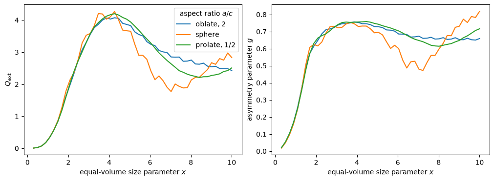
Averaged over orientations, spheroids follow the broad course of the sphere’s extinction but damp its interference structure, the large oscillation in \(x\) and the ripple on it. At a single size they can therefore differ from the equal-volume sphere by tens of percent, most where the sphere’s extinction peaks.

The phase matrix: what shape changes

The angular scattering differs much more. At \(x = 5\), the phase matrix of the three particles, normalized so that \(F_{11}\) averages to 1 over the sphere of directions. For a sphere \(F_{22} = F_{11}\); a spheroid’s \(F_{22}\) falls below \(F_{11}\), which depolarizes linearly polarized light. A backscatter lidar measures both effects: the linear depolarization ratio \(\delta = (F_{11} - F_{22})/(F_{11} + F_{22})\) at 180°, and the lidar ratio \(S = 4\pi/(\omega F_{11})\) at 180°, with \(\omega\) the single-scattering albedo.

angles = np.linspace(0, 180, 361)
mu = np.cos(np.radians(angles))
f = tmatrix.phase_matrix(5.0, m, shapes, mu)  # each element of shape (3, 361)
q5 = tmatrix.efficiencies(5.0, m, shapes)
albedo = q5.q_sca / q5.q_ext
depolarization = (f.f11[:, -1] - f.f22[:, -1]) / (f.f11[:, -1] + f.f22[:, -1])
lidar_ratio = 4 * np.pi / (albedo * f.f11[:, -1])
for e, d, s in zip(shapes, depolarization, lidar_ratio, strict=True):
    print(f"a/c = {e:3.1f}: depolarization {d:5.3f}, lidar ratio {s:5.1f} sr")
assert np.allclose(f.f22[1], f.f11[1], rtol=1e-9, atol=0) and abs(depolarization[1]) < 1e-9
assert np.all(depolarization[[0, 2]] > 0.2) and np.all(lidar_ratio[[0, 2]] > 2 * lidar_ratio[1])

a/c = 2.0: depolarization 0.451, lidar ratio  58.2 sr
a/c = 1.0: depolarization -0.000, lidar ratio  17.7 sr
a/c = 0.5: depolarization 0.232, lidar ratio  68.9 sr

fig, axes = plt.subplots(1, 3, figsize=(12, 3.6), layout="constrained")
for i, label in enumerate(["oblate, 2", "sphere", "prolate, 1/2"]):
    axes[0].semilogy(angles, f.f11[i], label=label)
    axes[1].plot(angles, -f.f12[i] / f.f11[i], label=label)
    axes[2].plot(angles, f.f22[i] / f.f11[i], label=label)
axes[0].set(ylabel="$F_{11}$")
axes[1].set(ylabel="$-F_{12}/F_{11}$ (degree of linear polarization)")
axes[2].set(ylabel="$F_{22}/F_{11}$")
for ax in axes:
    ax.set(xlabel="scattering angle (°)", xticks=[0, 45, 90, 135, 180])
axes[0].legend(title="aspect ratio $a/c$")
plt.show()

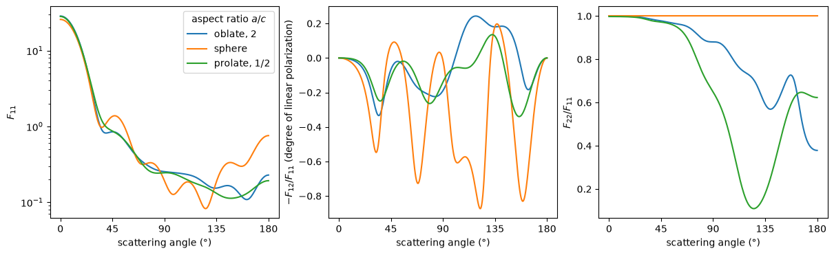
Both spheroids scatter three to four times less light straight back than the sphere, which raises the lidar ratio from about 18 sr to 60–70 sr, and their depolarization ratios are 0.23 and 0.45 where the sphere’s is zero.

A mixture of shapes

Natural dust is a mixture of shapes. The phase matrix of a mixture is the average of its members’ weighted by their scattering cross sections: with normalized=False the phase matrices are already multiplied by \(Q_\text{sca}\), and since every member has the same volume here, they average directly. Fifteen aspect ratios from 1/3 to 3, evenly spaced in \(\ln(a/c)\) and equally numerous, against the sphere, all of one size here; the next section averages over sizes too.

mixture = np.geomspace(1 / 3, 3, 15)
fm = tmatrix.phase_matrix(5.0, m, mixture, mu, normalized=False)
qm = tmatrix.efficiencies(5.0, m, mixture)
f11, f22 = fm.f11.mean(axis=0) / qm.q_sca.mean(), fm.f22.mean(axis=0) / qm.q_sca.mean()
albedo_mix = qm.q_sca.mean() / qm.q_ext.mean()
d_mix = (f11[-1] - f22[-1]) / (f11[-1] + f22[-1])
s_mix = 4 * np.pi / (albedo_mix * f11[-1])
print(f"mixture: depolarization {d_mix:.3f}, lidar ratio {s_mix:.1f} sr")
# The average is still normalized, ½∫F11 dμ = 1: each F11 is a polynomial in μ of degree 2N,
# which a Gauss–Legendre rule of 64 nodes integrates exactly.
nodes, weights = scatrs.special.gauss_legendre(64)
f_nodes = tmatrix.phase_matrix(5.0, m, mixture, nodes, normalized=False)
assert abs(weights @ f_nodes.f11.mean(axis=0) / qm.q_sca.mean() / 2 - 1) < 1e-12

fig, (ax1, ax2) = plt.subplots(1, 2, figsize=(10, 3.6), layout="constrained")
ax1.semilogy(angles, f.f11[1], color="0.5", label="sphere")
ax1.semilogy(angles, f11, label="mixture of spheroids")
ax2.plot(angles, (f.f11[1] - f.f22[1]) / (f.f11[1] + f.f22[1]), color="0.5", label="sphere")
ax2.plot(angles, (f11 - f22) / (f11 + f22), label="mixture of spheroids")
ax1.set(ylabel="$F_{11}$")
ax2.set(ylabel="$(F_{11} - F_{22})/(F_{11} + F_{22})$")
for ax in (ax1, ax2):
    ax.set(xlabel="scattering angle (°)", xticks=[0, 45, 90, 135, 180])
ax1.legend()
plt.show()

mixture: depolarization 0.220, lidar ratio 43.8 sr

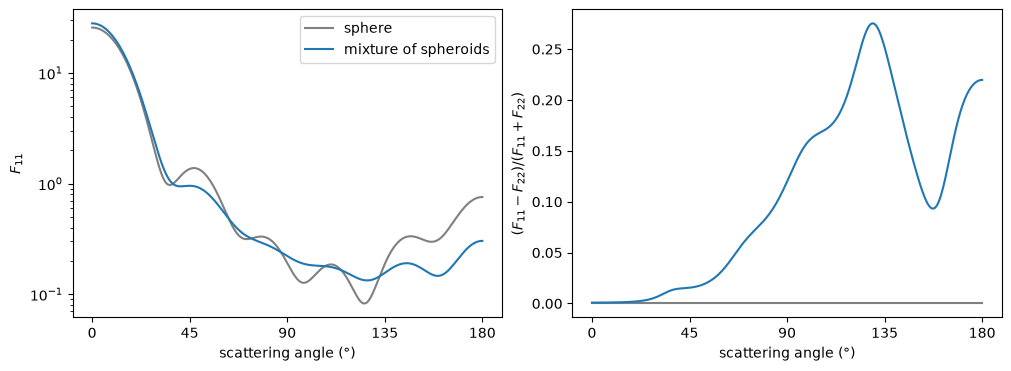
The mixture smooths the single shapes’ features into a flat side and back scattering, with a depolarization of about 0.2 and a lidar ratio near 45 sr, of the order lidars measure in desert dust.

Size distributions and mixtures of shapes

An Ensemble of Spheroid particles averages over a size distribution as for spheres (Example: an aerosol size distribution); its size is the radius of the sphere of equal volume. A Mixture of ensembles of different aspect ratios is a mixture of shapes, weighted as the previous section weighted them by hand. Each size node solves a T-matrix, so an ensemble of spheroids costs seconds where spheres cost milliseconds, and the tighter rtol, the further the integration reaches into the large sizes of the distribution’s tail; a loose rtol such as \(10^{-4}\) keeps it practical (Ensembles). A dust mode at 550 nm, four shapes in equal numbers (this cell takes about half a minute):

size = scatrs.LogNormal(median_radius=0.15, width=1.4)  # µm
shapes = [1 / 3, 1 / 2, 2.0, 3.0]
dust = scatrs.Mixture([(1.0, scatrs.Ensemble(scatrs.Spheroid(m, e), size)) for e in shapes])
spheres = scatrs.Ensemble(scatrs.Sphere(m), size)
options = {"rtol": 1e-4, "greek": 16, "mu": [-1.0]}
rd, rs = dust.compute(0.55, **options), spheres.compute(0.55, **options)
for name, r in [("spheroids", rd), ("spheres", rs)]:
    print(f"{name:9}: C_ext {r.c_ext:.4e} µm² (± {r.error.c_ext:.0e}), g {r.g:.4f}, "
          f"lidar ratio {r.lidar_ratio:.1f} sr, depolarization {r.depolarization:.3f}")
assert rd.converged and rs.depolarization == 0 and rd.depolarization > 0.05
assert rd.lidar_ratio > 1.2 * rs.lidar_ratio
# A sphere's F22 is its F11; a mixture of spheroids' is not.
assert rs.phase.f22 == rs.phase.f11 and rd.phase.f22 < rd.phase.f11

spheroids: C_ext 1.8810e-01 µm² (± 4e-06), g 0.6884, lidar ratio 105.8 sr, depolarization 0.108
spheres  : C_ext 2.0057e-01 µm² (± 4e-06), g 0.6722, lidar ratio 74.9 sr, depolarization 0.000

Particles comparable to the wavelength: the spheroids extinguish about 6% less than spheres of the same volume, scatter more forward, and scatter less straight back, which raises the lidar ratio from about 75 to about 105 sr and depolarizes the backscattered light by about 0.1.

Greek coefficients

For radiative transfer, tmatrix.greek expands the phase matrix in generalized spherical functions, as mie.greek does for spheres (Example: phase matrix and Greek coefficients), but with the six expansions independent: \(F_{22}\) and \(F_{44}\) no longer follow from the others. Normalized, \(\alpha_1^0 = 1\) and \(\alpha_1^1 = 3g\), and the expansion is exact at order \(2N\), beyond which every coefficient is zero.

g = tmatrix.greek(5.0, m, 2.0)
print(f"orders 0..{len(g.alpha1) - 1} (N = {int(g.n_terms)}); "
      f"alpha1[1] / 3 = {g.alpha1[1] / 3:.12f}, g = {q5.g[0]:.12f}")
assert g.alpha1[0] == 1 and abs(g.alpha1[1] / 3 - q5.g[0]) < 1e-12

fig, ax = plt.subplots(figsize=(6, 3.6), layout="constrained")
for name in ("alpha1", "alpha2", "alpha3", "alpha4", "beta1", "beta2"):
    ax.semilogy(abs(getattr(g, name)) + 1e-17, ".-", label=name)
ax.set(xlabel="order $l$", ylabel="|coefficient|", ylim=(1e-16, 10))
ax.legend(ncols=2, fontsize=8)
plt.show()

orders 0..36 (N = 18); alpha1[1] / 3 = 0.727937107845, g = 0.727937107845

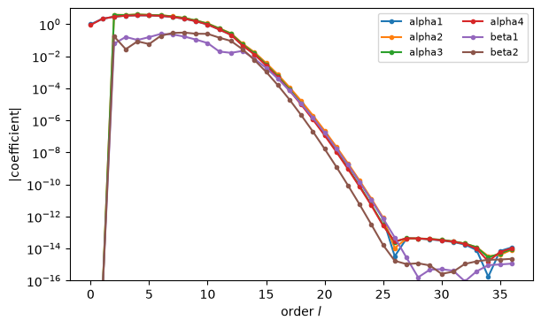
The coefficients fall steeply past order 10 and reach the level of rounding, about \(10^{-14}\) of the first ones, near order 26; the expansion stops at \(2N = 36\).

Convergence, error estimates and precision

Each spheroid’s T-matrix is converged to the tolerance rtol (default \(10^{-8}\)) in its number of orders \(N\) and of quadrature nodes \(n_\theta\), and every result carries both and an error estimate per spheroid. The results of the first section:

print(f"N from {q.n_terms.min()} to {q.n_terms.max()}, n_theta from {q.n_theta.min()} to "
      f"{q.n_theta.max()}, largest estimated error {q.error.max():.1e}")
assert np.all(q.error < 1e-8)

N from 7 to 38, n_theta from 16 to 83, largest estimated error 9.4e-09

tmatrix.compute returns the T-matrix of one spheroid as an object, with its convergence information and its outputs. For elongated spheroids the integrals behind the T-matrix lose precision in double precision; scatrs solves the modes that need it with mixed-precision refinement, and reports how it solved each one (precision_paths). Here a prolate spheroid of \(a/c = 1/3\) at \(x = 8\):

t = tmatrix.compute(8.0, m, 1 / 3)
print(t, Counter(t.precision_paths))
assert t.converged and t.error_estimate < 1e-8

TMatrix(n_terms=40, n_modes=35, n_theta=88, error_estimate=8.3e-10) Counter({'f64': 28, 'refined': 7})

precision="f64" skips the refinement and "double-double" computes everything in double-double; the default "auto" refines only the modes whose estimate needs it. At this spheroid’s \(N\) and \(n_\theta\), against the double-double result:

fixed = {"n_terms": t.n_terms, "n_theta": t.n_theta}
reference = tmatrix.compute(8.0, m, 1 / 3, precision="double-double", **fixed).efficiencies()
print(f"{'precision':<15}{'estimate':>10}{'Q_ext error':>13}{'Q_sca error':>13}")
for precision in ("f64", "auto"):
    s = tmatrix.compute(8.0, m, 1 / 3, precision=precision, **fixed)
    e = s.efficiencies()
    errors = [abs(e.q_ext / reference.q_ext - 1), abs(e.q_sca / reference.q_sca - 1)]
    print(f"{precision:<15}{s.error_estimate:10.1e}{errors[0]:13.1e}{errors[1]:13.1e}")
    assert max(errors) <= s.error_estimate

precision        estimate  Q_ext error  Q_sca error

f64               6.9e-05      1.0e-09      9.5e-10

auto              8.3e-10      7.8e-16      2.1e-15

The estimates bound the errors; in double precision alone the bound is \(10^{-4}\), too large for the default tolerance, which is why the default refines. precision="f64" is the fastest, for tolerances its estimate meets.

The T-matrix itself

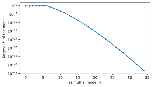
block(m) returns the T-matrix of azimuthal mode \(m\), whose orders run from \(\max(m, 1)\) to \(N\). Its elements fall steeply with the mode, so the modes above a cutoff, whose elements fall below rtol/10 of the largest, contribute nothing measurable and are not computed: n_modes says how many were, and block raises IndexError above them.

modes = np.arange(t.n_modes)
largest = []
for mm in modes:
    b = t.block(mm)
    largest.append(max(abs(v).max() for v in (b.t11, b.t12, b.t21, b.t22)))
print(f"N = {t.n_terms}, modes computed: {t.n_modes}; mode 0: orders "
      f"{t.block(0).orders[0]}..{t.block(0).orders[-1]}, largest element {largest[0]:.2f}; "
      f"mode 20: {largest[20]:.1e}")
assert t.n_modes <= t.n_terms + 1 and largest[20] < 1e-12 * largest[0]

fig, ax = plt.subplots(figsize=(6, 3.4), layout="constrained")
ax.semilogy(modes, largest, ".-")
ax.set(xlabel="azimuthal mode $m$", ylabel="largest $|T|$ of the mode")
plt.show()

N = 40, modes computed: 35; mode 0: orders 1..40, largest element 0.56; mode 20: 4.1e-19

Derivatives

derivatives=True returns the derivatives with respect to "x", "aspect_ratio", "m_real" and "m_imag", in closed form; d(name) selects one. They are what a retrieval of size, shape or composition needs. Here the sensitivity of an oblate spheroid’s extinction to its aspect ratio, against a central difference of results at a tight tolerance:

qd = tmatrix.efficiencies(3.0, m, 2.0, derivatives=True)
h = 1e-5
up, down = (tmatrix.efficiencies(3.0, m, 2.0 + s * h, rtol=1e-12) for s in (1, -1))
difference = (up.q_ext - down.q_ext) / (2 * h)
print(f"dQ_ext/d(a/c): {qd.d('aspect_ratio').q_ext:.10f}, central difference {difference:.10f}")
print(f"dQ_ext/dx {qd.d('x').q_ext:.4f}, dQ_abs/d(Im m) {qd.d('m_imag').q_abs:.4f}")
assert abs(qd.d("aspect_ratio").q_ext - difference) < 1e-7 * abs(difference)

dQ_ext/d(a/c): -0.1020276480, central difference -0.1020276481
dQ_ext/dx 1.3138, dQ_abs/d(Im m) 13.8055

Outside the validated domain

The validated domain covers aspect ratios from 1/5 to 5, equal-volume \(x \ge 10^{-6}\), \(|m|\,x_{\max} \le 60\), \(1.3 \le \mathrm{Re}\,m \le 3\) and \(\mathrm{Im}\,m \le 0.5\) (Internal validation). Outside it a call raises OutsideValidatedDomainError, unless allow_unvalidated=True: then it computes as usual, with its error estimate, but without a declared accuracy. A needle of \(a/c = 1/10\):

try:
    tmatrix.efficiencies(1.0, m, 0.1)
except scatrs.OutsideValidatedDomainError as error:
    print(error)
needle = tmatrix.efficiencies(1.0, m, 0.1, allow_unvalidated=True)
print(f"Q_ext = {needle.q_ext:.10f}, N = {needle.n_terms}, n_theta = {needle.n_theta}, "
      f"estimate {needle.error:.1e}")
assert needle.error < 1e-8

outside validated domain: element 0: aspect ratio 0.1, x = 1, m = 1.53+0.008i
Q_ext = 0.1633150019, N = 18, n_theta = 75, estimate 1.3e-09

Elongated and flattened spheroids need many quadrature nodes, set by their shape rather than by \(N\) (Spheroids). External validation checks such spheroids, up to a silver nanorod with \(a/c = 1/20\), against published values computed in arbitrary precision.