Example: Mie scattering by spheres

scatrs.mie computes the Mie coefficients, efficiencies and amplitudes of homogeneous spheres, vectorized over size parameter and refractive index, with derivatives. This page runs whenever the documentation is built; its checks are asserts, so a failing check fails the build.

import matplotlib.pyplot as plt
import numpy as np

from scatrs import mie

# Water droplets in visible light, from Rayleigh to geometric optics.
x = np.geomspace(0.01, 1000, 9)
q = mie.efficiencies(x, 1.33 + 1e-8j)
for xi, qe, w, g in zip(x, q.q_ext, q.q_sca / q.q_ext, q.g, strict=True):
    print(f"x = {xi:8.2f}   Q_ext = {qe:.4e}   single-scattering albedo = {w:.10f}   g = {g:+.4f}")

x =     0.01   Q_ext = 1.3346e-09   single-scattering albedo = 0.8316172923   g = +0.0000
x =     0.04   Q_ext = 3.5188e-07   single-scattering albedo = 0.9973051783   g = +0.0003
x =     0.18   Q_ext = 1.1073e-04   single-scattering albedo = 0.9999634836   g = +0.0058
x =     0.75   Q_ext = 3.2715e-02   single-scattering albedo = 0.9999993919   g = +0.1022
x =     3.16   Q_ext = 1.9488e+00   single-scattering albedo = 0.9999999334   g = +0.7942
x =    13.34   Q_ext = 2.1612e+00   single-scattering albedo = 0.9999997171   g = +0.7227
x =    56.23   Q_ext = 2.2345e+00   single-scattering albedo = 0.9999986049   g = +0.8372
x =   237.14   Q_ext = 2.0740e+00   single-scattering albedo = 0.9999959114   g = +0.8751
x =  1000.00   Q_ext = 2.0166e+00   single-scattering albedo = 0.9999830375   g = +0.8831

From Rayleigh to geometric optics

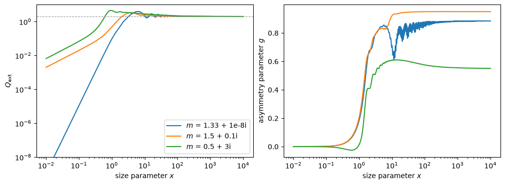
The efficiencies across six decades of size parameter, for a weakly absorbing water droplet, a strongly absorbing sphere and a metal-like one. Small spheres scatter like \(x^4\) (Rayleigh) and absorb like \(x\); the extinction of the weak absorber then oscillates (the broad interference structure, with fine resonance ripples on top) and settles on 2 for large spheres. The asymmetry parameter \(g\) rises from 0 as the scattering turns forward.

xs = np.geomspace(0.01, 1e4, 4000)
cases = {"1.33 + 1e-8i": 1.33 + 1e-8j, "1.5 + 0.1i": 1.5 + 0.1j, "0.5 + 3i": 0.5 + 3j}

fig, (ax1, ax2) = plt.subplots(1, 2, figsize=(10, 3.6), layout="constrained")
for label, m in cases.items():
    q = mie.efficiencies(xs, m)
    (line,) = ax1.loglog(xs, q.q_ext, label=f"$m$ = {label}")
    ax2.semilogx(xs, q.g, color=line.get_color())
ax1.axhline(2, color="0.6", lw=0.8, ls="--")
ax1.set(xlabel="size parameter $x$", ylabel="$Q_\\mathrm{ext}$", ylim=(1e-8, 10))
ax2.set(xlabel="size parameter $x$", ylabel="asymmetry parameter $g$")
ax1.legend()
plt.show()

Extinction paradox and the optical theorem

Large spheres remove twice their geometric cross section (\(Q_\text{ext} \to 2\)), and \(Q_\text{ext}\) equals \((4/x^2)\,\mathrm{Re}\,S(0)\), the optical theorem, which scatrs does not use to compute it.

q = mie.efficiencies(1e4, 1.5 + 0.01j)
s = mie.amplitudes(1e4, 1.5 + 0.01j, 1.0)
print(q.q_ext, 4 / 1e4**2 * s.s1.real)
assert abs(q.q_ext - 2) < 0.01
assert abs(4 / 1e4**2 * s.s1.real / q.q_ext - 1) < 1e-11

2.0042876782829895 2.0042876782829997

Weak absorption without cancellation

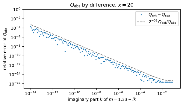
For weakly absorbing particles, \(Q_\text{abs} = Q_\text{ext} - Q_\text{sca}\) cancels: here 4, 6 and 8 digits for \(k = 10^{-6}\), \(10^{-8}\) and \(10^{-10}\). scatrs computes \(Q_\text{abs}\) from an exact per-term identity instead (Homogeneous spheres (Lorenz–Mie)), so the co-albedo \(1 - \omega = Q_\text{abs}/Q_\text{ext}\) keeps full precision. For small \(k\), \(Q_\text{abs}/k\) is linear in \(k\): the direct value at \(k = 10^{-10}\) matches the linear extrapolation from \(k = 10^{-6}\) and \(10^{-8}\) to about 10 digits, and the difference misses it in the 8th.

direct, by_difference = {}, {}
for k in (1e-6, 1e-8, 1e-10):
    q = mie.efficiencies(20.0, 1.33 + 1j * k)
    direct[k], by_difference[k] = q.q_abs / k, (q.q_ext - q.q_sca) / k
    print(f"k = {k:.0e}: Q_abs/k direct {direct[k]:.15f}, by difference {by_difference[k]:.15f}")
slope = (direct[1e-6] - direct[1e-8]) / (1e-6 - 1e-8)
linear = direct[1e-8] - slope * (1e-8 - 1e-10)
print(f"relative distance from the extrapolation at k = 1e-10: "
      f"direct {abs(direct[1e-10] / linear - 1):.1e}, "
      f"by difference {abs(by_difference[1e-10] / linear - 1):.1e}")
assert abs(direct[1e-10] / linear - 1) < 1e-9

k = 1e-06: Q_abs/k direct 97.755046150969193, by difference 97.755046151171143
k = 1e-08: Q_abs/k direct 97.761847356601507, by difference 97.761847372979105
k = 1e-10: Q_abs/k direct 97.761915375293029, by difference 97.761914119587345
relative distance from the extrapolation at k = 1e-10: direct 6.8e-11, by difference 1.3e-08

Over a range of absorption, the difference loses about \(\log_{10}(Q_\text{ext}/Q_\text{abs})\) digits, which the direct value does not (here measured against it).

k = np.geomspace(1e-14, 1e-1, 200)
q = mie.efficiencies(20.0, 1.33 + 1j * k)
loss = np.abs((q.q_ext - q.q_sca) / q.q_abs - 1)

fig, ax = plt.subplots(figsize=(6, 3.4), layout="constrained")
ax.loglog(k, np.maximum(loss, 1e-17), ".", ms=3, label="$Q_\\mathrm{ext} - Q_\\mathrm{sca}$")
ax.loglog(k, 2.0**-52 * q.q_ext / q.q_abs, "--", color="0.5",
          label="$2^{-52}\\,Q_\\mathrm{ext}/Q_\\mathrm{abs}$")
ax.set(xlabel="imaginary part $k$ of $m = 1.33 + ik$", ylabel="relative error of $Q_\\mathrm{abs}$",
       title="$Q_\\mathrm{abs}$ by difference, $x = 20$", ylim=(1e-17, 1))
ax.legend()
plt.show()

The phase function

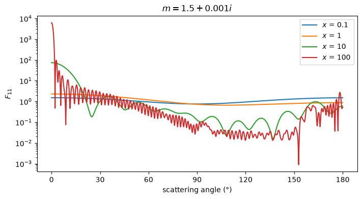
The phase function \(F_{11}\) is \((\lvert S_1\rvert^2 + \lvert S_2\rvert^2)/2\) divided by \(x^2 Q_\text{sca}/4\), which normalizes it so that \(\tfrac12\int_{-1}^1 F_{11}\,d\mu = 1\) (Conventions). It turns from the symmetric Rayleigh shape into a narrow forward peak, with a glory in the backward direction, as the sphere grows.

angle = np.linspace(0, 180, 1801)
mu = np.cos(np.radians(angle))

fig, ax = plt.subplots(figsize=(7, 3.8), layout="constrained")
for x0 in (0.1, 1, 10, 100):
    s = mie.amplitudes(x0, 1.5 + 0.001j, mu)
    q = mie.efficiencies(x0, 1.5 + 0.001j)
    f11 = (abs(s.s1) ** 2 + abs(s.s2) ** 2) / 2 / (x0**2 * q.q_sca / 4)
    ax.semilogy(angle, f11, label=f"$x$ = {x0:g}")
ax.set(xlabel="scattering angle (°)", ylabel="$F_{11}$", title="$m = 1.5 + 0.001i$",
       xticks=range(0, 181, 30))
ax.legend()
plt.show()

\(F_{11}\) is a polynomial of degree \(2N\) in \(\mu\), so a Gauss–Legendre rule with \(N + 1\) points integrates it exactly.

from scatrs.special import gauss_legendre

x0, m0 = 30.0, 1.5 + 0.001j
n = int(mie.default_n_max(x0))
mu, w = gauss_legendre(n + 1)
s = mie.amplitudes(x0, m0, mu)
q = mie.efficiencies(x0, m0)
f11 = (abs(s.s1) ** 2 + abs(s.s2) ** 2) / 2 / (x0**2 * q.q_sca / 4)
print("normalization:", 0.5 * np.sum(w * f11))
print("asymmetry parameter:", 0.5 * np.sum(w * f11 * mu), q.g)
assert abs(0.5 * np.sum(w * f11) - 1) < 1e-13
assert abs(0.5 * np.sum(w * f11 * mu) - q.g) < 1e-13

normalization: 1.0000000000000029
asymmetry parameter: 0.8164031902416009 0.8164031902415981

Derivatives

derivatives=True returns the derivatives with respect to the size parameter and the real and imaginary parts of the refractive index, in closed form, for 1.2 to 2.2 times the cost of the values. Here they are checked against central differences.

x0, m0 = 12.0, 1.45 + 0.02j
q = mie.efficiencies(x0, m0, derivatives=True)
h = 1e-6
for name, dq, at in [
    ("x", q.d("x"), lambda e: mie.efficiencies(x0 + e, m0)),
    ("m_real", q.d("m_real"), lambda e: mie.efficiencies(x0, m0 + e)),
    ("m_imag", q.d("m_imag"), lambda e: mie.efficiencies(x0, m0 + 1j * e)),
]:
    fd = (at(h).q_ext - at(-h).q_ext) / (2 * h)
    print(f"dQ_ext/d{name}: closed form {dq.q_ext:+.10f}, finite difference {fd:+.10f}")
    assert abs(dq.q_ext - fd) < 1e-7 * max(1, abs(fd))

dQ_ext/dx: closed form -0.0098261578, finite difference -0.0098261572
dQ_ext/dm_real: closed form +0.8824589736, finite difference +0.8824589735
dQ_ext/dm_imag: closed form -6.3233217781, finite difference -6.3233217771

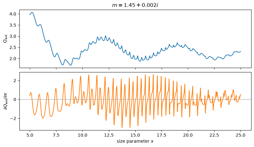
The derivatives are exact for the computed series, so they follow every resonance ripple of the extinction curve, where a finite difference would need a very small step.

xs = np.linspace(5, 25, 4001)
q = mie.efficiencies(xs, 1.45 + 0.002j, derivatives=["x"])
dq = q.d("x").q_ext

fig, (ax1, ax2) = plt.subplots(2, 1, figsize=(8, 4.6), sharex=True, layout="constrained")
ax1.plot(xs, q.q_ext)
ax1.set(ylabel="$Q_\\mathrm{ext}$", title="$m = 1.45 + 0.002i$")
ax2.plot(xs, dq, color="C1")
ax2.axhline(0, color="0.6", lw=0.8)
ax2.set(xlabel="size parameter $x$", ylabel="$\\partial Q_\\mathrm{ext}/\\partial x$")
plt.show()