Example: size distributions and refractive-index models

An Ensemble is a particle and a size distribution. This page goes through the seven size distributions of scatrs.size, and how much the optics depend on the distribution’s form, then through the refractive-index models of scatrs.refractive that let a particle’s index vary with wavelength, and the derivatives with respect to a model’s parameters. See Ensembles and Refractive-index models for the definitions. This page runs whenever the documentation is built; its checks are asserts, so a failing check fails the build. Radii and wavelengths are in µm.

import matplotlib.pyplot as plt
import numpy as np

import scatrs
from scatrs import refractive


def angstrom(wavelength, c_ext):
    """The Ångström exponent −d ln C_ext/d ln λ between neighbouring wavelengths."""
    return -np.diff(np.log(c_ext)) / np.diff(np.log(wavelength))

One effective radius, five distributions

Hansen & Travis (1974) showed that the scattering of a size distribution depends mostly on two of its moments: the effective radius \(r_\text{eff} = \langle r^3\rangle/\langle r^2\rangle\) and the effective variance \(v_\text{eff} = \langle (r - r_\text{eff})^2 r^2\rangle/(r_\text{eff}^2\langle r^2\rangle)\). Water droplets with \(r_\text{eff} = 1\) µm and \(v_\text{eff} = 0.1\), in five forms:

• Gamma, Hansen & Travis’s gamma distribution, takes the two directly.

• ModifiedGamma, Deirmendjian’s \(r^\alpha e^{-b r^\gamma}\), is the same distribution for \(\gamma = 1\), \(\alpha = 1/v_\text{eff} - 3\) and \(b = 1/(r_\text{eff}v_\text{eff})\).

• Tabulated takes the same density at 400 radii, interpolated linearly.

• LogNormal has the same two moments for \(\sigma_g = \exp\sqrt{\ln(1 + v_\text{eff})}\) and \(r_g = r_\text{eff}/(1 + v_\text{eff})^{5/2}\).

• Monodisperse droplets of radius \(r_\text{eff}\), the limit \(v_\text{eff} = 0\).

The distributions’ mean cross sections differ, so they are compared by efficiency, the mean extinction cross section over the mean geometric one, \(\bar Q_\text{ext} = \langle C_\text{ext}\rangle/\langle\pi r^2\rangle\).

r_eff, v_eff = 1.0, 0.1
radius = np.linspace(0.01, 4.0, 400)
distributions = {
    "Gamma": scatrs.Gamma(effective_radius=r_eff, effective_variance=v_eff),
    "ModifiedGamma": scatrs.ModifiedGamma(alpha=1 / v_eff - 3, b=1 / (r_eff * v_eff), gamma=1.0),
    "Tabulated": scatrs.Tabulated(radius, radius ** (1 / v_eff - 3) * np.exp(-radius / (r_eff * v_eff))),
    "LogNormal": scatrs.LogNormal(
        median_radius=r_eff / (1 + v_eff) ** 2.5, width=np.exp(np.sqrt(np.log(1 + v_eff)))
    ),
    "Monodisperse": scatrs.Monodisperse(radius=r_eff),
}
water = scatrs.Sphere(1.33 + 1e-8j)
wavelength = np.array([0.4, 0.55, 0.87, 1.6])
angles = np.linspace(0, 180, 361)
results = {
    name: scatrs.Ensemble(water, d).compute(wavelength, mu=np.cos(np.radians(angles)))
    for name, d in distributions.items()
}
q_ext = {name: r.c_ext / r.mean_area for name, r in results.items()}
print(f"{'':14}{'r_eff':>9}" + "".join(f"{'Q_ext ' + str(w):>12}" for w in wavelength))
for name, r in results.items():
    print(f"{name:14}{r.effective_radius[0]:9.5f}" + "".join(f"{v:12.5f}" for v in q_ext[name]))
gamma = results["Gamma"]
assert np.allclose(q_ext["ModifiedGamma"], q_ext["Gamma"], rtol=1e-6, atol=0)
assert np.allclose(q_ext["Tabulated"], q_ext["Gamma"], rtol=1e-4, atol=0)
assert np.allclose(q_ext["LogNormal"], q_ext["Gamma"], rtol=0.03, atol=0)
assert np.all(abs(results["LogNormal"].g - gamma.g) < 0.01)
assert np.max(abs(q_ext["Monodisperse"] / q_ext["Gamma"] - 1)) > 0.2

                  r_eff   Q_ext 0.4  Q_ext 0.55  Q_ext 0.87   Q_ext 1.6
Gamma           1.00000     2.34936     2.51536     3.20376     2.52241
ModifiedGamma   1.00000     2.34936     2.51536     3.20376     2.52241
Tabulated       1.00003     2.34937     2.51532     3.20370     2.52250
LogNormal       1.00000     2.31998     2.50559     3.26263     2.51032
Monodisperse    1.00000     2.84290     1.80088     3.74607     2.74412

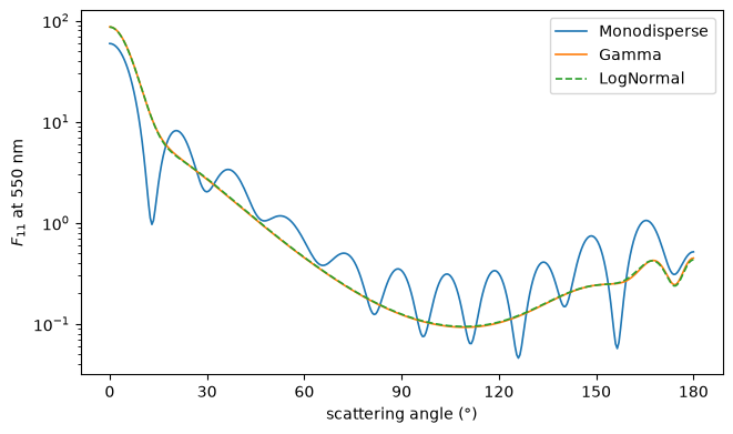
The modified gamma distribution reproduces the gamma one, and the table it within its interpolation error. The lognormal of the same two moments differs by under 2% in extinction and 0.005 in \(g\); the single size, by tens of percent. The phase functions at 550 nm show why: a single size has the sharp oscillations of interference, which any spread of sizes smooths away, and the two distributions of the same moments are hard to tell apart.

fig, ax = plt.subplots(figsize=(6.5, 3.8), layout="constrained")
for name, style in [("Monodisperse", "-"), ("Gamma", "-"), ("LogNormal", "--")]:
    ax.semilogy(angles, results[name].phase.f11[1], style, label=name, lw=1.2)
ax.set(xlabel="scattering angle (°)", ylabel="$F_{11}$ at 550 nm", xticks=range(0, 181, 30))
ax.legend()
plt.show()

A power law

PowerLaw is \(n(r) \propto r^{-\alpha}\) between two radii, as Junge’s distribution of continental aerosol. Where its bounds do not matter, the extinction of \(n(r) \propto r^{-4}\) falls as \(\lambda^{-1}\): its Ångström exponent is \(\alpha - 3 = 1\).

lam = np.array([0.4, 0.5, 0.6, 0.7, 0.87])
junge = scatrs.Ensemble(
    scatrs.Sphere(1.45 + 1e-3j), scatrs.PowerLaw(exponent=4.0, min_radius=0.02, max_radius=10.0)
).compute(lam)
print("Ångström exponents:", np.round(angstrom(lam, junge.c_ext), 3))
print(f"effective radius {junge.effective_radius[0]:.3f} µm")
assert np.all(abs(angstrom(lam, junge.c_ext) - 1) < 0.05)

Ångström exponents: [1.005 1.008 1.011 1.014]
effective radius 0.125 µm

Several modes

MultiModal adds distributions, each normalized, with weights: the fractions of the particles in each mode. Atmospheric aerosol is often a fine mode with a few coarse particles, here one in a thousand. They are few in number but large, so they carry much of the extinction and flatten its spectrum.

fine = scatrs.LogNormal(median_radius=0.08, width=1.6)
coarse = scatrs.LogNormal(median_radius=1.0, width=1.8)
particle = scatrs.Sphere(1.45 + 1e-3j)
fine_only = scatrs.Ensemble(particle, fine).compute(lam)
bimodal = scatrs.Ensemble(particle, scatrs.MultiModal([(0.999, fine), (0.001, coarse)])).compute(lam)
coarse_share = 1 - 0.999 * fine_only.c_ext / bimodal.c_ext
print("Ångström, fine mode:", np.round(angstrom(lam, fine_only.c_ext), 2))
print("Ångström, bimodal:  ", np.round(angstrom(lam, bimodal.c_ext), 2))
print("coarse share of the extinction:", np.round(coarse_share, 2))
assert np.all(angstrom(lam, bimodal.c_ext) < angstrom(lam, fine_only.c_ext))

Ångström, fine mode: [1.7  2.02 2.27 2.52]
Ångström, bimodal:   [1.25 1.31 1.26 1.08]
coarse share of the extinction: [0.22 0.29 0.38 0.47 0.61]

Distribution parameters given as arrays make a grid of distributions, computed at once, as Example: an aerosol size distribution shows for an optics table.

Refractive-index models

A number given to a particle is a constant index. For an index that varies with wavelength, scatrs.refractive has four models: a dispersion law, Sellmeier or Cauchy; a Table of measured values; and any Function of the wavelength.

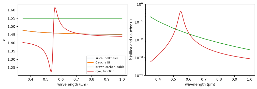
A dispersion law and its range. Fused silica follows a three-term Sellmeier law (Malitson 1965) from the ultraviolet to the infrared. A Cauchy law \(n = A + B/\lambda^2\) through its values at 450 and 650 nm follows it closely in the visible, but not beyond.

silica = refractive.Sellmeier(
    B=[0.6961663, 0.4079426, 0.8974794],
    C=[0.0684043**2, 0.1162414**2, 9.896161**2],
)
n1, n2 = silica.evaluate([0.45, 0.65]).real
B = (n1 - n2) / (1 / 0.45**2 - 1 / 0.65**2)
cauchy = refractive.Cauchy(A=n1 - B / 0.45**2, B=B)
visible = np.linspace(0.4, 0.7, 31)
print(f"Cauchy: A = {cauchy.A:.6f}, B = {cauchy.B:.6f} µm²")
print(f"largest difference 400–700 nm: {np.max(abs(cauchy.evaluate(visible) - silica.evaluate(visible))):.1e}")
print(f"difference at 2 µm: {abs(cauchy.evaluate(2.0) - silica.evaluate(2.0)):.1e}")
assert np.max(abs(cauchy.evaluate(visible) - silica.evaluate(visible))) < 2e-4

Cauchy: A = 1.448223, B = 0.003512 µm²
largest difference 400–700 nm: 9.7e-05
difference at 2 µm: 1.1e-02

A table, interpolated. Absorption that changes by decades between the tabulated wavelengths, such as brown carbon’s, which falls steeply with wavelength, is interpolated better in \(\ln k\) than in \(k\). Here \(k = 0.03\,(0.55/\lambda)^4\) tabulated every 100 nm:

def brown_carbon(wl):
    return 1.55 + 0.03j * (0.55 / np.asarray(wl)) ** 4


nodes = np.linspace(0.3, 1.0, 8)
fine_grid = np.linspace(0.3, 1.0, 141)
k_exact = brown_carbon(fine_grid).imag
for interpolation in ("linear", "log_k"):
    table = refractive.Table(nodes, brown_carbon(nodes), interpolation=interpolation)
    k_error = np.max(abs(table.evaluate(fine_grid).imag / k_exact - 1))
    print(f"{interpolation:>6}: largest relative error in k {k_error:.1%}")
log_table = refractive.Table(nodes, brown_carbon(nodes), interpolation="log_k")
assert np.max(abs(log_table.evaluate(fine_grid).imag / k_exact - 1)) < 0.05

linear: largest relative error in k 22.4%
 log_k: largest relative error in k 4.2%

A table is not extrapolated: outside its wavelengths it raises.

try:
    log_table.evaluate(1.2)
except scatrs.InvalidInputError as error:
    print(error)

invalid input: wavelength 1.2 is outside the Table's range [0.3, 1.0]

A function. Any callable of the wavelength is a model. An absorption band, from a Lorentz oscillator (Bohren & Huffman 1983, Chapter 9) at 550 nm: the permittivity is \(\varepsilon = \varepsilon_\infty + f\omega_0^2/(\omega_0^2 - \omega^2 - i\gamma\omega)\) in wavenumbers \(\omega = 1/\lambda\), and \(m = \sqrt\varepsilon\).

def lorentz_band(wl):
    w, w0 = 1 / np.asarray(wl), 1 / 0.55  # wavenumbers, 1/µm
    epsilon = 2.0 + 0.05 * w0**2 / (w0**2 - w**2 - 0.08j * w)
    return np.sqrt(epsilon)


dye = refractive.Function(lorentz_band)
spectrum = np.linspace(0.35, 1.0, 131)
fig, (ax1, ax2) = plt.subplots(1, 2, figsize=(10, 3.4), layout="constrained")
for label, model in [("silica, Sellmeier", silica), ("Cauchy fit", cauchy),
                     ("brown carbon, table", log_table), ("dye, function", dye)]:
    m = model.evaluate(spectrum)
    ax1.plot(spectrum, m.real, label=label)
    ax2.semilogy(spectrum, np.maximum(m.imag, 1e-6), label=label)
ax1.set(xlabel="wavelength (µm)", ylabel="$n$")
ax2.set(xlabel="wavelength (µm)", ylabel="$k$ (silica and Cauchy: 0)", ylim=(1e-4, 1))
ax1.legend(fontsize=8)
plt.show()

In an ensemble the model is evaluated at the wavelengths computed, and the values used are in the result’s refractive_index. Small dye particles absorb most in the band, near 550 nm:

dyed = scatrs.Ensemble(scatrs.Sphere(dye), scatrs.LogNormal(median_radius=0.05, width=1.5))
r = dyed.compute(spectrum)
assert np.array_equal(r.refractive_index, dye.evaluate(spectrum))
peak = spectrum[np.argmax(r.c_abs)]
print(f"C_abs peaks at {peak:.3f} µm")
assert 0.5 < peak < 0.6

C_abs peaks at 0.550 µm

Derivatives with respect to a model’s parameters

An ensemble’s derivatives with respect to "m_real" and "m_imag" are those with respect to \(\mathrm{Re}\,m\) and \(\mathrm{Im}\,m\) at each wavelength, whatever model produced \(m\). A model’s derivatives(wavelength) gives \(\partial m/\partial\theta\) for each of its parameters, and the chain rule combines the two: for the Cauchy law’s \(A\), $\partial C/\partial A = \partial C/\partial,\mathrm{Re},m;\mathrm{Re},\partial m/\partial A

• \partial C/\partial,\mathrm{Im},m;\mathrm{Im},\partial m/\partial A$.

glass = scatrs.LogNormal(median_radius=0.1, width=1.5)
r = scatrs.Ensemble(scatrs.Sphere(cauchy), glass).compute(wavelength, derivatives=["m_real", "m_imag"])
dm_dA = cauchy.derivatives(wavelength)[cauchy.parameters.index("A")]
dc_dA = r.d("m_real").c_ext * dm_dA.real + r.d("m_imag").c_ext * dm_dA.imag

h = 1e-6
shifted = [
    scatrs.Ensemble(scatrs.Sphere(refractive.Cauchy(A=cauchy.A + s * h, B=cauchy.B)), glass)
    .compute(wavelength, rtol=1e-10).c_ext
    for s in (1, -1)
]
difference = (shifted[0] - shifted[1]) / (2 * h)
print("dC_ext/dA:         ", dc_dA)
print("central difference:", difference)
assert np.allclose(dc_dA, difference, rtol=1e-6, atol=0)

dC_ext/dA:          [0.24879674 0.18120434 0.06735072 0.00982658]
central difference: [0.24879673 0.18120434 0.06735072 0.00982658]