External validation¶

The internal validation (Internal validation) shows that scatrs evaluates the Mie equations accurately. This page checks that it evaluates the right equations, in the conventions users expect, against results that do not depend on scatrs’s code: the published test cases of another Mie code, and the limits of known physics. The page runs whenever the documentation is built; its checks are asserts, so a failing check fails the build.

Wiscombe’s MIEV0 test cases¶

Wiscombe’s MIEV0 (Wiscombe 1979, 1980) is the most widely used Mie code, and its documentation publishes test cases that most Mie codes since have been checked against: \(Q_\text{ext}\), \(Q_\text{sca}\), and the amplitudes \(S_1\) and \(S_2\) at seven angles from 0° to 180°, to seven significant digits. The cases span small and large spheres, refractive indices below 1, weak and strong absorption, and a metal-like \(m = 10 + 10i\).

MIEV0 uses time dependence \(e^{+i\omega t}\): its refractive index is written \(n - ik\), and its amplitudes are the complex conjugates of scatrs’s (Conventions). The values are those of test cases 5 to 19, as tabulated in the test suite of sasktran2, which replaces a few backward-angle amplitudes at \(x = 10^4\) (cases 11, 16 and 19) with values from another code; those are left out here.

import json
from pathlib import Path

import matplotlib.pyplot as plt
import numpy as np

from scatrs import mie

data = json.loads(Path("data", "miev0-test-cases.json").read_text())
mu = np.cos(np.radians(data["angles_deg"]))


def half_unit(printed):
    """Half a unit in the last printed digit of a number such as "2.101321E+00" or "0.093923"."""
    mantissa, _, exponent = printed.upper().partition("E")
    decimals = len(mantissa.partition(".")[2])
    return 0.5 * 10.0 ** (int(exponent or 0) - decimals)


rows = []
for case in data["cases"]:
    x, m = case["x"], complex(*case["m"])
    q = mie.efficiencies(x, m)
    s = mie.amplitudes(x, m, mu)
    # Amplitude differences relative to the amplitudes' size: the larger of |S| and its
    # root-mean-square value over all directions, x √Q_sca / 2.
    scale_rms = x * np.sqrt(q.q_sca) / 2
    worst_s = max(
        abs(got - complex(*want).conjugate()) / max(abs(complex(*want)), scale_rms)
        for name, values in (("s1", s.s1), ("s2", s.s2))
        for got, want in zip(values, case[name], strict=True)
        if want is not None
    )
    # Q differences in units of the last printed digit.
    worst_q = max(abs(getattr(q, k) - float(case[k])) / (2 * half_unit(case[k]))
                  for k in ("q_ext", "q_sca") if k in case)
    rows.append((case["case"], x, m, q.q_ext, q.q_sca, worst_q, worst_s))

print(f"{'case':>4} {'x':>8} {'m':>12} {'Q_ext':>10} {'Q_sca':>10} "
      f"{'Q: last digits':>15} {'S: relative':>12}")
for c, x, m, qe, qs, dq, ds in rows:
    print(f"{c:4d} {x:8g} {f'{m.real:g}+{m.imag:g}i':>12} {qe:10.7f} {qs:10.7f} {dq:15.2f} {ds:12.1e}")
assert max(r[5] for r in rows) < 1, "a Q differs by a unit in its last printed digit"
assert max(r[6] for r in rows) < 1e-6, "an amplitude differs in its 7th digit"

case        x            m      Q_ext      Q_sca  Q: last digits  S: relative
  0.099      0.75+0i  0.0000074  0.0000074            0.42      8.3e-07
  0.101      0.75+0i  0.0000080  0.0000080            0.03      6.9e-07
     10      0.75+0i  2.2322648  2.2322648            0.16      3.2e-07
   1000      0.75+0i  1.9979082  1.9979082            0.18      9.2e-08
      1  1.33+1e-05i  0.0939520  0.0939233            0.37      3.1e-07
    100  1.33+1e-05i  2.1013207  2.0965935            0.49      6.9e-08
  10000  1.33+1e-05i  2.0040889  1.7238572            0.22      7.7e-08
  0.055       1.5+1i  0.1014910  0.0000113            0.42      9.8e-08
  0.056       1.5+1i  0.1033467  0.0000122            0.16      8.2e-08
      1       1.5+1i  2.3363210  0.6634538            0.38      1.2e-07
    100       1.5+1i  2.0975018  1.2836970            0.24      1.1e-07
  10000       1.5+1i  2.0043677  1.2365743            0.69      7.8e-08
      1       10+10i  2.5329931  2.0494050            0.08      7.7e-08
    100       10+10i  2.0711243  1.8367854            0.40      7.5e-08
  10000       10+10i  2.0059143  1.7953930            0.33      8.2e-08

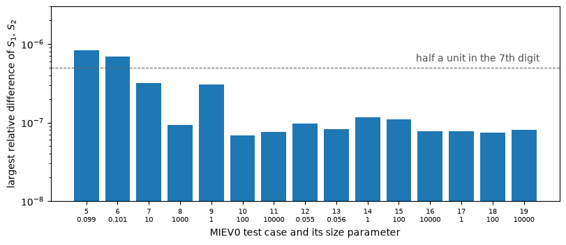
Every published \(Q\) is reproduced to within one unit in its last printed digit (the column “Q: last digits”), and every amplitude to within \(10^{-6}\) of the amplitudes’ size. All but two cases agree to within half a unit in the seventh digit, the rounding of the published values. The two exceptions, cases 5 and 6 at \(x \approx 0.1\), differ by less than \(10^{-6}\); there the declared accuracy of scatrs’s amplitudes is better than \(10^{-12}\) (Internal validation), so the differences come from the published values.

cases = [r[0] for r in rows]
fig, ax = plt.subplots(figsize=(8, 3.4), layout="constrained")
ax.bar(np.arange(len(rows)), [r[6] for r in rows], color="C0")
ax.axhline(5e-7, color="0.4", ls="--", lw=0.8)
ax.text(len(rows) - 0.5, 6e-7, "half a unit in the 7th digit", ha="right", color="0.3")
ax.set_xticks(np.arange(len(rows)), [f"{c}\n{r[1]:g}" for c, r in zip(cases, rows, strict=True)],
              fontsize=7)
ax.set(yscale="log", ylim=(1e-8, 3e-6), xlabel="MIEV0 test case and its size parameter",
       ylabel="largest relative difference of $S_1$, $S_2$")
plt.show()

../_images/eca5aea0445aa90e8eeb2cafddea4f229790bed040ae10a6c32a532f5c7126ec.png

Rayleigh scattering¶

Spheres much smaller than the wavelength scatter as dipoles. Their scattering efficiency is \(Q_\text{sca} = \tfrac83 x^4 \lvert (m^2 - 1)/(m^2 + 2)\rvert^2\), with corrections of order \(x^2\), and their normalized phase matrix has the closed form \(F_{11} = \tfrac34(1 + \mu^2)\), \(F_{12} = -\tfrac34(1 - \mu^2)\), \(F_{33} = \tfrac32\mu\), \(F_{34} = 0\). Its Greek coefficients (Mishchenko, Travis & Lacis 2002) are \(\alpha_1 = (1, 0, \tfrac12)\), \(\alpha_2^2 = 3\), \(\alpha_4^1 = \tfrac32\) and \(\beta_1^2 = -\sqrt6/2\), all others zero. These fix the sign convention of every element: a sign error in any of them would show here.

x_small = 1e-4
for m in (1.33, 1.5 + 0.1j, 0.5 + 3j, 10 + 10j):
    q = mie.efficiencies(x_small, m)
    rayleigh = 8 / 3 * x_small**4 * abs((m * m - 1) / (m * m + 2)) ** 2
    print(f"m = {m}: Q_sca / Rayleigh - 1 = {q.q_sca / rayleigh - 1:+.1e}")
    assert abs(q.q_sca / rayleigh - 1) < 1e-6

mu_check = np.linspace(-1, 1, 11)
f = mie.phase_matrix(x_small, 1.5, mu_check)
for got, want in [
    (f.f11, 0.75 * (1 + mu_check**2)),
    (f.f12, -0.75 * (1 - mu_check**2)),
    (f.f33, 1.5 * mu_check),
    (f.f34, 0 * mu_check),
]:
    assert np.allclose(got, want, rtol=0, atol=1e-7)

g = mie.greek(x_small, 1.5, 4)
expected = {
    "alpha1": [1, 0, 0.5, 0, 0], "alpha2": [0, 0, 3, 0, 0], "alpha3": [0, 0, 0, 0, 0],
    "alpha4": [0, 1.5, 0, 0, 0], "beta1": [0, 0, -np.sqrt(6) / 2, 0, 0], "beta2": [0, 0, 0, 0, 0],
}
for name, want in expected.items():
    print(f"{name}: {np.round(getattr(g, name), 6) + 0.0}")  # + 0.0: no negative zeros
    assert np.allclose(getattr(g, name), want, rtol=0, atol=1e-7), name

m = 1.33: Q_sca / Rayleigh - 1 = -7.4e-10
m = (1.5+0.1j): Q_sca / Rayleigh - 1 = +7.4e-10
m = (0.5+3j): Q_sca / Rayleigh - 1 = +1.8e-08
m = (10+10j): Q_sca / Rayleigh - 1 = +1.2e-08
alpha1: [1.  0.  0.5 0.  0. ]
alpha2: [0. 0. 3. 0. 0.]
alpha3: [0. 0. 0. 0. 0.]
alpha4: [0.  1.5 0.  0.  0. ]
beta1: [ 0.        0.       -1.224745  0.        0.      ]
beta2: [0. 0. 0. 0. 0.]

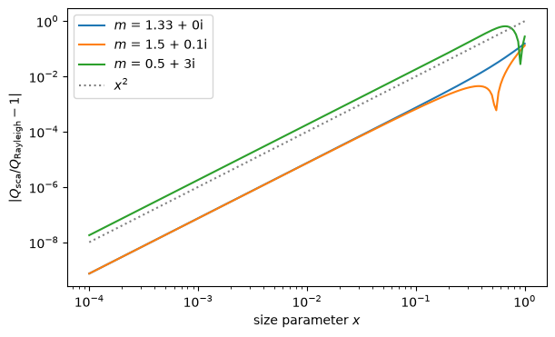
As \(x\) grows, \(Q_\text{sca}\) leaves the Rayleigh law by a relative amount proportional to \(x^2\):

xs = np.geomspace(1e-4, 1, 200)
fig, ax = plt.subplots(figsize=(6, 3.6), layout="constrained")
for m in (1.33 + 0j, 1.5 + 0.1j, 0.5 + 3j):
    q = mie.efficiencies(xs, m)
    rayleigh = 8 / 3 * xs**4 * abs((m * m - 1) / (m * m + 2)) ** 2
    ax.loglog(xs, abs(q.q_sca / rayleigh - 1), label=f"$m$ = {m.real:g} + {m.imag:g}i")
ax.loglog(xs, xs**2, ":", color="0.5", label="$x^2$")
ax.set(xlabel="size parameter $x$", ylabel="$|Q_\\mathrm{sca}/Q_\\mathrm{Rayleigh} - 1|$")
ax.legend()
plt.show()

../_images/2921dd1cf27bc706cc23da6244f6da21693038ed05c807b98098f9e413623ade.png

Large spheres and the optical theorem¶

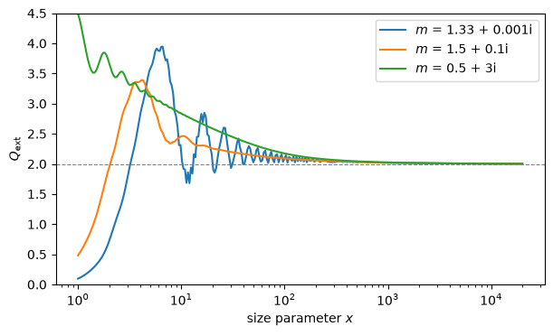
A sphere much larger than the wavelength removes twice its geometric cross section, half by absorption or reflection and refraction and half by diffraction (the extinction paradox), so \(Q_\text{ext} \to 2\). And for every sphere, the extinction equals the forward amplitude by the optical theorem, \(Q_\text{ext} = (4/x^2)\,\mathrm{Re}\,S(0°)\). scatrs computes \(Q_\text{ext}\) from the Mie coefficients directly, not through \(S(0°)\), so the two are independent results.

xs = np.geomspace(1, 2e4, 300)
fig, ax = plt.subplots(figsize=(6, 3.6), layout="constrained")
for m in (1.33 + 1e-3j, 1.5 + 0.1j, 0.5 + 3j):
    q = mie.efficiencies(xs, m)
    s = mie.amplitudes(xs, m, 1.0)
    theorem = 4 / xs**2 * s.s1.real
    assert np.allclose(theorem, q.q_ext, rtol=1e-10, atol=0)
    ax.semilogx(xs, q.q_ext, label=f"$m$ = {m.real:g} + {m.imag:g}i")
    assert abs(q.q_ext[-1] - 2) < 0.02
ax.axhline(2, color="0.5", ls="--", lw=0.8)
ax.set(xlabel="size parameter $x$", ylabel="$Q_\\mathrm{ext}$", ylim=(0, 4.5))
ax.legend()
plt.show()

../_images/52d51397d0ec48e2ebd2aa20ff1e36bb1ae29186d23edecfcee53d155d7ba0a5.png

A non-absorbing sphere conserves energy: \(Q_\text{abs}\) is exactly zero, and \(Q_\text{ext} = Q_\text{sca}\).

q = mie.efficiencies(np.geomspace(1e-3, 1e4, 50), 1.33)
assert np.all(q.q_abs == 0)
assert np.allclose(q.q_ext, q.q_sca, rtol=1e-13, atol=0)

Layered spheres¶

A layered sphere has its own checks from physics, which do not depend on any code.

An air shell changes nothing. A shell of the medium’s own index (\(m = 1\)) around a core is not there: the coefficients are the bare core’s. scatrs computes them from the shell’s functions at both radii, so the check exercises the whole recursion.

from scatrs import layered

for x_core, m_core in [(0.5, 1.5 + 0.01j), (12.0, 1.95 + 0.79j), (80.0, 1.33)]:
    core = mie.coefficients(x_core, m_core)
    n = int(core.n_terms)
    coated = layered.coefficients([x_core, 1.6 * x_core], [m_core, 1.0], n_max=n,
                                  allow_unvalidated=True)
    err = max(abs(coated.a[:n] - core.a).max(), abs(coated.b[:n] - core.b).max())
    scale = max(abs(core.a).max(), abs(core.b).max())
    print(f"x_core = {x_core:g}, m = {m_core}: relative difference {err / scale:.1e}")
    assert err <= 1e-12 * scale

x_core = 0.5, m = (1.5+0.01j): relative difference 1.7e-16
x_core = 12, m = (1.95+0.79j): relative difference 4.6e-15
x_core = 80, m = 1.33: relative difference 5.8e-15

Layers of one index are one sphere. Splitting a sphere into shells of its own index gives the homogeneous sphere of the outer radius, exactly:

q = layered.efficiencies([2.0, 5.0, 9.0], [1.5 + 0.01j] * 3)
q0 = mie.efficiencies(9.0, 1.5 + 0.01j)
assert q.q_ext == q0.q_ext and q.q_abs == q0.q_abs and q.g == q0.g

The Rayleigh limit. A coated sphere much smaller than the wavelength scatters as a dipole of the electrostatic polarizability of a coated sphere (Bohren & Huffman 1983, chapter 5): with \(\varepsilon = m^2\) of the core (1) and shell (2) and the core volume fraction \(f = (x_1/x_2)^3\), \(a_1 \to -\tfrac{2i}{3}x^3\,\tilde\alpha\) with

\[\tilde\alpha = \frac{(\varepsilon_2 - 1)(\varepsilon_1 + 2\varepsilon_2) + f(2\varepsilon_2 + 1)(\varepsilon_1 - \varepsilon_2)} {(\varepsilon_2 + 2)(\varepsilon_1 + 2\varepsilon_2) + 2f(\varepsilon_2 - 1)(\varepsilon_1 - \varepsilon_2)},\]

with corrections of order \(x^2\):

x_out = 1e-4
for m1, m2 in [(1.95 + 0.79j, 1.43 + 0.01j), (1.33, 10 + 10j), (0.2 + 3j, 1.45)]:
    for f_r in (0.1, 0.5, 0.9):
        e1, e2, f = m1 * m1, m2 * m2, f_r**3
        ratio = ((e2 - 1) * (e1 + 2 * e2) + f * (2 * e2 + 1) * (e1 - e2)) / (
            (e2 + 2) * (e1 + 2 * e2) + 2 * f * (e2 - 1) * (e1 - e2)
        )
        a1 = layered.coefficients([f_r * x_out, x_out], [m1, m2]).a[0]
        assert abs(a1 / (-2j / 3 * x_out**3 * ratio) - 1) < 10 * x_out**2
print("the Rayleigh limit holds to order x² for every case")

the Rayleigh limit holds to order x² for every case

Energy. A particle of real indices absorbs nothing, and for absorbing ones the extinction equals the forward amplitude (the optical theorem), computed independently:

q = layered.efficiencies([3.0, 6.0, 9.0], [1.5, 2.5, 1.33])
assert q.q_abs == 0 and q.q_ext == q.q_sca
x, m = [20.0, 35.0], [1.95 + 0.79j, 1.43 + 1e-8j]
q, s = layered.efficiencies(x, m), layered.amplitudes(x, m, 1.0)
assert abs(4 / 35.0**2 * s.s1.real / q.q_ext - 1) < 1e-12

Comparison with scattnlay¶

scattnlay (Peña & Pal 2009) computes layered spheres by the recursion scatrs builds on, in double precision. The script benchmarks/compare_scattnlay.py measures both, and the textbook method (direct matching at the interfaces in double precision, as Bohren & Huffman’s BHCOAT does), against the 362 Arb reference cases inside scatrs’s validated domain. The results it wrote are in benchmarks/results/2026-10-14-arm64-scattnlay.json. Apple M4 Pro, macOS; scatrs 0.2.0, scattnlay 2.4, 2026-10-14.

output	scatrs: largest error	scattnlay: cases above \(10^{-10}\), above \(10^{-6}\), failed	direct matching: the same
\(a_n\), \(b_n\)	\(2.9\cdot10^{-12}\)	118, 50, 9	143, 94, 43
\(Q_\text{ext}\)	\(4.1\cdot10^{-12}\)	102, 63, 6	157, 111, 59
\(Q_\text{sca}\)	\(4.1\cdot10^{-12}\)	100, 49, 6	151, 108, 59
\(Q_\text{abs}\)	\(6.3\cdot10^{-11}\)	174, 71, 6	205, 110, 53
\(Q_\text{back}\)	\(5.4\cdot10^{-11}\)	110, 46, 6	188, 109, 59
\(g\)	\(7.3\cdot10^{-12}\)	108, 55, 9	173, 131, 59
\(S_1\), \(S_2\)	\(9.3\cdot10^{-11}\)	140, 50, 6	142, 50, 0

The errors are measured as in Internal validation (relative, \(Q_\text{back}\) relative to the larger of \(Q_\text{back}\) and \(Q_\text{sca}\), \(g\) to the larger of \(|g|\) and \(10^{-3}\), the amplitudes to the larger of \(|S|\) and its RMS size); a failure is a missing or non-finite result. Where scattnlay disagrees, Arb sides with scatrs. Its errors have identifiable causes:

Absorption. scattnlay computes \(Q_\text{abs} = Q_\text{ext} - Q_\text{sca}\), which loses the digits of a weak absorption: a relative error of 2.4 for a core of index \(1.5 + 10^{-8}i\) in a clear shell at \(x_L = 1\). scatrs computes \(Q_\text{abs}\) directly (Layered spheres).
Very small particles. Below \(x \approx 10^{-3}\), scattnlay reduces its number of terms (“nmax value was changed due to unexpected error”) or fails, and its numerators lose the cancelling terms that scatrs removes.
Near-unity indices and air shells: for a small core in an air shell, errors of \(4\cdot10^{-7}\) in the coefficients and \(3\cdot10^{-4}\) in \(g\).

On one thread, scatrs computed the efficiencies of a coated sphere (black carbon in sulfate, core radius half the outer) 4.3 to 8.4 times faster:

\(x_L\)	scatrs (µs)	with every derivative (µs)	scattnlay (µs)
1	1.7	9.0	14.2
10	2.7	18.4	21.1
100	10.9	83.7	58.3
1000	104		451

Spheroids¶

Limits¶

A sphere. An aspect ratio of 1 gives every output of scatrs.mie, to \(10^{-9}\) or better (tests/test_tmatrix.py and scatrs/src/tmatrix/mod.rs).
The Rayleigh limit. At \(x = 0.01\) the orientation-averaged absorption and scattering of oblate and prolate spheroids (\(\varepsilon\) from 1/4 to 4, \(m = 1.5 + 0.1i\)) follow the electrostatic polarizabilities \(\alpha_j = V(m^2 - 1)/(1 + L_j(m^2 - 1))\) of their depolarization factors \(L_j\) (Bohren & Huffman 1983, §5.3) to \(10^{-3}\), the size of the first correction.
The long-wavelength expansion. Majić et al. (2019) derived the T-matrix elements of a spheroid in closed form to \(O(X^6)\), with \(X = kc\): the 15 elements of the dipoles, quadrupoles and octupoles of modes 0 to 2 that are not zero to that order, including the couplings between electric and magnetic multipoles. Their errors are \(O(X^7)\), so as the size halves, the relative error of \(|T|^2\) must fall 16-fold for the two dipolar elements and 4-fold for the others, and that of the averaged cross sections 16-fold. Between \(\tilde X\) = 0.08 and 0.04 (equal-volume size parameter), for prolate (\(c/a\) = 3) and oblate (\(c/a\) = 1/2 and 1/4) spheroids, absorbing or not, scatrs’s elements and cross sections approach them at exactly these rates (measured exponents 4.00 and 2.00, within 0.03; scatrs/tests/tmatrix_long_wavelength.rs). This checks every block of the low-order T-matrix against an independent derivation, beyond the leading term the Rayleigh limit checks.

Comparison with Mishchenko’s T-matrix code¶

Mishchenko’s extended-precision code for randomly oriented particles (tmq.lp.f, Mishchenko & Travis 1994; the “tmatd” of the literature) is the standard reference for spheroids. The script benchmarks/compare_tmatd.py fetches it from its page at NASA GISS (it is not redistributed here), builds it with gfortran after patches that change no computation (the input read from standard input, 16 printed digits, gfortran’s names for its quad-precision intrinsics), and compares it with scatrs at rtol = 1e-10 for 72 spheroids: aspect ratios 1/5, 1/3, 1/2, 2, 3 and 5, \(x\) = 1, 3, 6 and 10, and indices 1.33, \(1.53 + 0.008i\) and \(1.5 + 0.5i\). One particle is computed as the code’s notes describe, as a size distribution \(10^{-7}\) wide. The results are in benchmarks/results/2026-10-15-arm64-tmatd.json. Apple M4 Pro, macOS, both on one thread; scatrs 0.3.0, GNU Fortran 14.2, 2026-10-15.

output	at tmatd’s tolerance \(10^{-6}\): median, largest difference	at \(10^{-9}\): median, largest
\(Q_\text{ext}\)	\(1.6\cdot10^{-9}\), \(6.4\cdot10^{-8}\)	\(7.0\cdot10^{-13}\), \(7.5\cdot10^{-11}\)
\(Q_\text{sca}\)	\(2.1\cdot10^{-9}\), \(8.6\cdot10^{-8}\)	\(9.3\cdot10^{-13}\), \(6.8\cdot10^{-11}\)
\(g\)	\(1.2\cdot10^{-8}\), \(4.1\cdot10^{-8}\)	\(1.1\cdot10^{-8}\), \(3.7\cdot10^{-8}\)
Greek coefficients	\(3.6\cdot10^{-7}\), \(4.1\cdot10^{-6}\)	\(4.0\cdot10^{-8}\), \(2.9\cdot10^{-7}\)

The differences are relative (\(g\) absolute, the Greek coefficients relative to the largest \(\alpha_1\), normalized). They shrink with tmatd’s tolerance to the floor of its narrow size distribution, about \(10^{-8}\) in \(g\) and the Greek coefficients; scatrs’s own estimates are \(10^{-11}\) or below. tmatd expands \(F_{12}\) and \(F_{34}\) in the generalized spherical functions \(P^l_{02} = -d^l_{02}\), so its \(\beta_1\) and \(\beta_2\) have the opposite signs of scatrs’s, which uses the Wigner d-functions; the phase matrices agree.

tmatd stops (“convergence is not obtained”) for five spheroids: \(\varepsilon = 1/5\) at \(x = 10\) for every index, \(\varepsilon = 1/5\) at \(x = 6\) and \(\varepsilon = 5\) at \(x = 10\) for the absorbing index (at the tighter tolerance). There its number of orders grows to its limit of 140 without the cross sections settling: the loss of precision of the classical integrals, which scatrs removes (Spheroids). scatrs computes them with about 45 orders.

On one thread, the median time per spheroid, over the spheroids tmatd computes at both of its tolerances, scatrs at rtol \(10^{-6}\) and \(10^{-8}\), tmatd at \(10^{-6}\) and \(10^{-9}\):

\(x\)	scatrs, \(10^{-6}\) (s)	scatrs, \(10^{-8}\) (s)	tmatd, \(10^{-6}\) (s)	tmatd, \(10^{-9}\) (s)
1	0.005	0.006	0.028	0.046
3	0.017	0.023	0.086	0.19
6	0.052	0.073	0.31	0.48
10	0.60	1.0	1.1	1.8

scatrs at rtol \(10^{-8}\) is faster than tmatd at \(10^{-9}\) for every one of the 67 spheroids tmatd computes: by 5 to 11 times at \(x = 1\), 4 to 10 times at \(x = 3\), 1.6 to 10 times at \(x = 6\) and 1.2 to 4 times at \(x = 10\) (median 1.8). At \(x = 10\) the modes that need refinement in double-double take most of its time; the closest cases are the aspect ratios 1/3, 3 and 5 with the weakly absorbing indices. The slowest spheroid, \(\varepsilon = 1/5\) with the absorbing index, which tmatd cannot compute, takes 25 s. scatrs also runs its quadrature in parallel, with results that do not depend on the number of threads.

We thank M. I. Mishchenko, L. D. Travis and the NASA Goddard Institute for Space Studies for making the code publicly available; its references are listed in References.

Published arbitrary-precision values¶

Somerville, Auguié & Le Ru (2013) tabulate \(Q_\text{sca}\) and \(Q_\text{ext}\) of three randomly oriented prolate spheroids computed with the T-matrix and its inversion in arbitrary precision, to 15 digits. The values do not depend on any double-precision code. The three spheroids are model 1 of the benchmark of Kuik, de Haan & Hovenier (1992), a large spheroid, and a silver nanorod at its plasmon resonance, outside scatrs’s validated domain. The paper’s efficiencies are cross sections over the orientation-averaged projected area, \(S/4\) for a convex particle, and its size parameter is \(x_{\max} = kc\); scatrs’s efficiencies are over the cross section of the sphere of equal volume, so the conversion below multiplies by the ratio of the two areas.

from scatrs import tmatrix


def published(h, x_max, m, q_sca, q_ext, **options):
    """scatrs against the paper for a prolate spheroid of c/a = h: relative differences."""
    eps = 1 / h
    x = x_max * eps ** (2 / 3)
    e = np.sqrt(1 - eps**2)
    surface = 2 * np.pi * eps**2 * (1 + 1 / (eps * e) * np.arcsin(e))  # with c = 1
    ratio = surface / 4 / (np.pi * eps ** (4 / 3))
    q = tmatrix.efficiencies(x, m, eps, **options)
    return abs(q.q_sca / ratio / q_sca - 1), abs(q.q_ext / ratio / q_ext - 1), float(q.error)


k = 2 * np.pi * 1.33 / 2560  # the nanorod: a = 10 nm, c = 200 nm in a solvent of index 1.33
cases = {
    "Kuik et al. model 1": (4, 10.079368, 1.55 + 0.01j, 3.21290554203154, 3.36721292620919, {}),
    "silver nanorod": (20, 200 * k, np.sqrt(-318 + 48.5j) / 1.33, 2.91644692910476,
                       18.6590264036833, {"allow_unvalidated": True}),
}
for name, (h, x_max, m, q_sca, q_ext, options) in cases.items():
    d_sca, d_ext, est = published(h, x_max, m, q_sca, q_ext, rtol=1e-12, **options)
    print(f"{name:20} Q_sca {d_sca:.1e}  Q_ext {d_ext:.1e}  (estimate {est:.1e})")
    assert max(d_sca, d_ext) < 1e-13

Kuik et al. model 1  Q_sca 1.5e-14  Q_ext 8.9e-16  (estimate 1.0e-14)

silver nanorod       Q_sca 1.1e-15  Q_ext 2.7e-15  (estimate 1.8e-14)

spheroid	\(c/a\)	\(x_{\max}\)	\(m\)	scatrs: \(Q_\text{sca}\), \(Q_\text{ext}\)	SMARTIES’s double precision
Kuik et al. model 1	4	10.079368	\(1.55 + 0.01i\)	\(1.5\cdot10^{-14}\), \(9\cdot10^{-16}\)	\(6\cdot10^{-15}\), \(9\cdot10^{-15}\)
large	4	35	\(1.5 + 0.02i\)	\(4.4\cdot10^{-14}\), \(2\cdot10^{-15}\)	\(7.1\cdot10^{-5}\), \(2.6\cdot10^{-5}\)
silver nanorod	20	0.653	\(1.02 + 13.45i\)	\(1\cdot10^{-15}\), \(3\cdot10^{-15}\)	\(2.4\cdot10^{-12}\), \(1.2\cdot10^{-12}\)

The differences are relative to the published values, at rtol \(10^{-12}\) (the large spheroid at \(10^{-10}\)). The large spheroid takes about 20 s, so it is checked by the test large_prolate_spheroid of scatrs/tests/spheroid_published.rs (ignored by default) rather than on this page; the other two are checked by that file’s default tests as well. The last column is the same paper’s double-precision code, SMARTIES’s algorithm, against the same values. The paper’s albedo for the large spheroid, 0.718371249381958, is not the ratio of its own \(Q_\text{sca}\) and \(Q_\text{ext}\), 0.7183712495692; scatrs’s albedo agrees with the ratio to \(2\cdot10^{-14}\). The nanorod’s index and aspect ratio are far outside the validated domain, but with the default settings it converges as closely; at an aspect ratio of 20 the nodes are set by the shape rather than by \(N\) (Spheroids).

SMARTIES¶

SMARTIES (Somerville, Auguié & Le Ru 2016) computes spheroids in double precision with the algorithm of their 2013 paper, which avoids the cancellations of the classical integrals. Its code is not run here. Its paper reports the largest maximum size parameter \(x_{\max} = k\max(a, c)\) at which the orientation-averaged extinction still converged, for each index and aspect ratio. Its authors attribute the remaining limit to the matrix inversion in double precision, which extended precision would lift; scatrs’s mixed-precision refinement does that. Where the two overlap:

relative index	SMARTIES, largest \(x_{\max}\) (aspect ratio 2, 4)	scatrs, validated \(x_{\max} = 60/\lvert m\rvert\)
1.311	50 and 45 (oblate), 50 and 45 (prolate)	46
1.5	35 and 30	40
\(1.5 + 0.02i\)	40 and 30	40
2.5	16 and 12 (oblate), 18 and 12 (prolate)	24

scatrs’s validated domain ends where its cost, not its accuracy, grows: on its accuracy map the results stay within their tolerance up to \(|m|\,x_{\max} = 70\) (Internal validation). SMARTIES reaches aspect ratios up to 100 and metallic indices. They are outside scatrs’s validated domain: scatrs computes them with allow_unvalidated, as it does the nanorod above, but declares no accuracy constants there. The analytic expansion of its authors (above) checks the low-order T-matrix.

Size distributions¶

For averages over size distributions, Comparison with sasktran2 compares scatrs with the Mie integration of the sasktran2 radiative transfer model, for accuracy and speed.