Quick start
scatrs computes the optical properties of particles: single spheres with scatrs.mie,
layered spheres with scatrs.layered, randomly oriented spheroids with
scatrs.tmatrix, and size distributions and mixtures of spheres with
Ensemble and Mixture.
This page shows the main calls and the conventions to know before using the results. See
Installation to install the package.
Conventions at a glance
These are the points that most often trip up a comparison with another code. The full list is in Conventions.
Quantity |
Convention |
|---|---|
Refractive index |
\(m = n + ik\), with \(k \ge 0\) for absorbing particles (Bohren & Huffman). Codes that write \(m = n - ik\), such as MIEV0 and sasktran2, need the complex conjugate. A negative imaginary part raises |
Size |
|
Cross sections |
|
Angles |
Functions of angle take \(\mu = \cos\Theta\), with \(\Theta\) the scattering angle. |
Phase matrix |
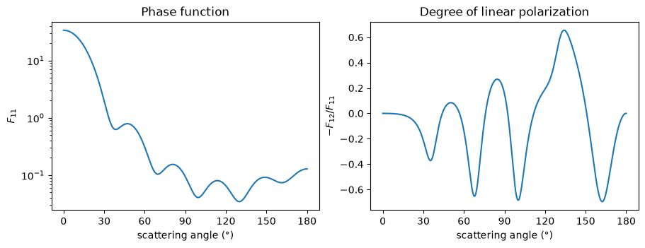
Normalized so that \(\tfrac12\int_{-1}^{1} F_{11}\,d\mu = 1\). The degree of linear polarization is \(-F_{12}/F_{11}\). |
Greek coefficients |
The expansion of Mishchenko, Travis & Lacis (2002), normalized so that \(\alpha_1^0 = 1\), and then \(\alpha_1^1 = 3g\). \(\beta_1\) and \(\beta_2\) have the opposite sign to sasktran2’s. |
Amplitudes |
\(S_1\), \(S_2\) of Bohren & Huffman, time dependence \(e^{-i\omega t}\): codes that use \(e^{+i\omega t}\), such as MIEV0, report their complex conjugates. |
Validated domain |
For spheres \(10^{-6} \le x \le 2\cdot10^4\), \(0 < \mathrm{Re}\,m \le 10\), \(0 \le \mathrm{Im}\,m \le 10\), \(\lvert m\rvert \ge 0.1\); layered spheres and spheroids have their own (Internal validation). Outside it, calls raise |
One sphere
A water droplet of radius 0.5 µm in green light. The functions take NumPy arrays (or scalars), which broadcast against each other.
import numpy as np

from scatrs import mie

radius, wavelength = 0.5, 0.55  # µm: any unit, the same for both
x = 2 * np.pi * radius / wavelength
m = 1.33 + 1e-8j

q = mie.efficiencies(x, m)
print(f"x = {x:.3f}")
print(f"Q_ext = {q.q_ext:.6f}, Q_sca = {q.q_sca:.6f}, Q_abs = {q.q_abs:.3e}")
print(f"single-scattering albedo = {q.q_sca / q.q_ext:.10f}, g = {q.g:.6f}")
print(f"C_ext = {q.q_ext * np.pi * radius**2:.6f} µm²")
x = 5.712
Q_ext = 3.926392, Q_sca = 3.926392, Q_abs = 2.537e-07
single-scattering albedo = 0.9999999354, g = 0.855569
C_ext = 3.083781 µm²
Angular scattering
phase_matrix() returns \(F_{11}\), \(F_{12}\), \(F_{33}\) and \(F_{34}\) at the
given cosines.
import matplotlib.pyplot as plt

angle = np.linspace(0, 180, 721)
f = mie.phase_matrix(x, m, np.cos(np.radians(angle)))

fig, (ax1, ax2) = plt.subplots(1, 2, figsize=(9, 3.4), layout="constrained")
ax1.semilogy(angle, f.f11)
ax1.set(xlabel="scattering angle (°)", ylabel="$F_{11}$", title="Phase function")
ax2.plot(angle, -f.f12 / f.f11)
ax2.set(xlabel="scattering angle (°)", ylabel="$-F_{12}/F_{11}$", title="Degree of linear polarization")
for ax in (ax1, ax2):
    ax.set_xticks(range(0, 181, 30))
plt.show()
Coefficients for radiative transfer
greek() expands the phase matrix in Wigner d-functions. The coefficients
are exact up to rounding, and by default every nonzero order is returned.
g = mie.greek(x, m)
print(f"{g.alpha1.shape[-1]} orders")
print("alpha1[:4] =", g.alpha1[:4])
print("beta1[:4]  =", g.beta1[:4])
assert g.alpha1[0] == 1 and abs(g.alpha1[1] - 3 * q.g) < 1e-12
41 orders
alpha1[:4] = [1.         2.56670747 3.67171735 4.2214725 ]
beta1[:4]  = [0.         0.         0.02885596 0.08311873]
A spheroid
scatrs.tmatrix computes randomly oriented spheroids by the T-matrix method, with the
outputs of scatrs.mie and two more elements of the phase matrix, \(F_{22}\) and \(F_{44}\),
which a sphere’s fixes (\(F_{22} = F_{11}\), \(F_{44} = F_{33}\)). A spheroid of semi-axes
\(a, a, c\) has aspect_ratio \(= a/c\), oblate above 1 and prolate below; x and the
efficiencies are those of the sphere of equal volume. Each result is converged to a tolerance
(rtol, by default \(10^{-8}\)) and carries its error estimate. The droplet above, flattened to
twice as wide as it is tall:
from scatrs import tmatrix

s = tmatrix.efficiencies(x, m, aspect_ratio=2.0)
print(f"Q_ext = {s.q_ext:.6f}, g = {s.g:.6f} (the sphere: {q.q_ext:.6f}, {q.g:.6f})")
print(f"N = {s.n_terms}, estimated error {s.error:.0e}")
f2 = tmatrix.phase_matrix(x, m, 2.0, np.cos(np.radians([90, 180])))
print("F22/F11 at 90° and 180°:", f2.f22 / f2.f11)
Q_ext = 3.730448, g = 0.853196 (the sphere: 3.926392, 0.855569)
N = 19, estimated error 4e-11
F22/F11 at 90° and 180°: [0.93736482 0.54815268]
A size distribution
An Ensemble is a particle and a size distribution;
compute() averages over the sizes at each wavelength. Every output comes
with an error estimate, and converged says whether the size integration met its tolerance
(rtol, by default \(10^{-6}\)).
import scatrs

sulfate = scatrs.Ensemble(
    scatrs.Sphere(refractive_index=1.43 + 1e-8j),
    scatrs.LogNormal(median_radius=0.08, width=1.6),  # µm
)
wavelengths = np.array([0.35, 0.55, 1.0])  # µm
r = sulfate.compute(wavelengths, greek=32)

for i, lam in enumerate(wavelengths):
    print(f"λ = {lam} µm: C_ext = {r.c_ext[i]:.4e} µm² (± {r.error.c_ext[i]:.0e}), "
          f"ω = {r.ssa[i]:.8f}, g = {r.g[i]:.4f}")
print("converged:", r.converged)
print("alpha1 at 0.55 µm:", r.greek.alpha1[1, :4])
λ = 0.35 µm: C_ext = 5.6498e-02 µm² (± 2e-08), ω = 0.99999994, g = 0.7165
λ = 0.55 µm: C_ext = 2.5967e-02 µm² (± 1e-08), ω = 0.99999993, g = 0.6340
λ = 1.0 µm: C_ext = 5.9044e-03 µm² (± 2e-09), ω = 0.99999986, g = 0.4419
converged: [ True  True  True]
alpha1 at 0.55 µm: [1.         1.90209946 1.89458392 1.33455216]
A refractive index that varies with wavelength is a model from scatrs.refractive, such
as a table of measured values (Refractive-index models). A
LayeredSphere is a core in concentric shells, such as black carbon coated in
sulfate, with the core’s radius 60% of the particle’s:
scatrs.LayeredSphere.coated(1.95 + 0.79j, 1.43 + 1e-8j, core_fraction=0.6)
(Example: coated black carbon). A Mixture combines
ensembles of different materials. Distribution parameters given as arrays make a grid of
distributions, computed at once, as an optics table needs:
table = scatrs.Ensemble(
    scatrs.Sphere(1.43 + 1e-8j),
    scatrs.LogNormal(median_radius=np.geomspace(0.05, 0.5, 4)[:, None], width=[1.4, 1.6, 1.8]),
)
t = table.compute(wavelengths)
print(t)
print("C_ext of r_g = 0.05 µm, σ_g = 1.6:", t.c_ext[0, 1])
EnsembleResult(shape=(4, 3, 3), params=(), grid=('median_radius', 'width'), converged=36/36)
C_ext of r_g = 0.05 µm, σ_g = 1.6: [0.00976992 0.0032902  0.00053417]
Derivatives
derivatives=True adds derivatives of every output, in closed form, at little extra cost:
with respect to the size parameter and the real and imaginary parts of the refractive index
for single spheres, and to the distribution parameters and the particle’s refractive indices
(and a layered sphere’s radius fractions) for ensembles.
q = mie.efficiencies(x, m, derivatives=True)
print("dQ_ext/dx       =", q.d("x").q_ext)
print("dQ_ext/d(Re m)  =", q.d("m_real").q_ext)

r = sulfate.compute(0.55, derivatives=["median_radius"])
print("dC_ext/dr_g =", r.d("median_radius").c_ext, "µm")
dQ_ext/dx       = 0.17050080312106897
dQ_ext/d(Re m)  = 6.222419712655691
dC_ext/dr_g = 1.3209486365224252 µm
Next steps
The examples go further: Example: Mie scattering by spheres, Example: phase matrix and Greek coefficients, Example: an aerosol size distribution, Example: size distributions and refractive-index models, Example: coated black carbon and Example: mineral dust as spheroids.
How scatrs is validated explains how the results are checked, and how far they can be trusted.
Python API documents every function and option.